RNN + Attentionで英語から日本語の機械翻訳を行う。
はじめに
Tensorflow のチュートリアルにあった、RNN+Attention の機械翻訳のモデルを勉強した。
この記事では、このチュートリアルを参考に、英語日本語の機械翻訳の AI を実装する。また Attention レイヤーを可視化も行う。
コードの全体は以下に配置した。この記事では重要な部分だけ解説する。
データ
データはこの記事と同じものを用いる。具体的なデータの加工方法についてはそちらを参考いただきたい。
Encoder と Decoder には以下のようなデータセットで学習する。
input_1: starttoken, this, is, a, pen, endtoken
input_2: starttoken, これ, は, ペン, です
output: これ, は, ペン, です, endtoken
前の記事との違いとして、input_1 に starttoken と endtoken を追加した。これは tensorflow のチュートリアルに合わせている。
モデルの構築
以下のコードでは次のようなハイパーパラメーターを用いる。これらのパラメーターは tensorflow のチュートリアルに習って設定した。
VOCAB_SIZE=20000
ENGLISH_SEQUENCE_LENGTH=16
JAPANESE_SEQUENCE_LENGTH=16
HIDDEN_DIM=512
EMBEDDING_DIM=512
BATCH_SIZE=512
Encoder
エンコーダーは次のように構築した。
class Encoder(Model):
    def __init__(self):
        super().__init__()
        self.embedding = Embedding(VOCAB_SIZE, EMBEDDING_DIM)
        self.gru = GRU(HIDDEN_DIM, return_sequences=True, return_state=True, recurrent_initializer='glorot_uniform')

    def call(self, inputs_1):
        x = self.embedding(inputs_1)
        sequences, last_sequence = self.gru(x, initial_state=None)
        return sequences, last_sequence
RNN の Encoder として基本的なものである。sequencesは途中の出力を全て含む文全体のテンソルであり、last_sequenceは最後の出力である。これらのテンソルの次元は次のようになる。
sequences: (BATCH_SIZE, ENGLISH_SEQUENCE_LENGTH, HIDDEN_DIM)
last_sequence: (BATCH_SIZE, HIDDEN_DIM)
last_sequenceはsequences[:, -1]に一致する。
Attention レイヤー
Attention レイヤーは次のように構築した。(これは tensorflow のチュートリアルと同じものである。)
class BahdanauAttention(Layer):
  def __init__(self, units):
    super(BahdanauAttention, self).__init__()
    self.W1 = tf.keras.layers.Dense(units)
    self.W2 = tf.keras.layers.Dense(units)
    self.V = tf.keras.layers.Dense(1)

  def call(self, query, values):
    hidden_with_time_axis = tf.expand_dims(query, 1)
    score = self.V(tf.nn.tanh(self.W1(values) + self.W2(hidden_with_time_axis)))
    attention_weights = tf.nn.softmax(score, axis=1)
    context_vector = attention_weights * values
    context_vector = tf.reduce_sum(context_vector, axis=1)
    return context_vector, attention_weights
このレイヤーの内部構造については、tensorflow のチュートリアルの説明に譲る。この記事ではこのレイヤーの使い方と解釈について重点をおいて説明する。このレイヤーは次のように用いる。
attention_layer = BahdanauAttention(HIDDEN_DIM)

for (english_batch, _), _ in train_dataset.take(1):
    sequences, last_sequence = encoder(english_batch)
    hidden_state = last_sequence
    context_vector, attention_weights = attention_layer(hidden_state, sequences)
    print(context_vector.shape, attention_weights.shape)
今回の機械翻訳において Attention は、Decoder の RNN の出力を用いて、Encoder が取り出した文全体のテンソルから、情報を取り出すのに用いられる。その際には、Decoder の潜在ベクトル(hidden_state)を query として設定し、Encoder の出力(sequences)の values から情報を取り出す。
Attention の入力の次元は次のようになる。
hidden_state (query): (BATCH_SIZE, HIDDEN_DIM)
sequences (values): (BATCH_SIZE, ENGLISH_SEQUENCE_LENGTH, HIDDEN_DIM)
これによって次のような次元のテンソルが出力される。
output: (BATCH_SIZE, HIDDEN_DIM)
attention_weights: (BATCH_SIZE, ENGLISH_SEQUENCE_LENGTH, 1)
Attention の output は query と同じ次元となる。また、attention_weights は output が Encoder の sequences のどの単語と強く結びついているのかを表す値となる。attention_weights を可視化することで単語同士の関係を可視化できる。
Decoder
Decoder は次のように構築した。
class Decoder(Model):
    def __init__(self):
        super(Decoder, self).__init__()
        self.embedding = Embedding(VOCAB_SIZE, EMBEDDING_DIM)
        self.gru = GRU(HIDDEN_DIM, return_sequences=True, return_state=True, recurrent_initializer='glorot_uniform')
        self.attention = BahdanauAttention(HIDDEN_DIM)
        self.dense = Dense(VOCAB_SIZE)

    def call(self, dec_input, hidden_state, sequences):
        x = self.embedding(dec_input)
        outputs = []
        attentions = []

        for t in range(JAPANESE_SEQUENCE_LENGTH):
            context_vector, attention_score = self.attention(hidden_state, sequences)
	    decoder_inputs = context_vector + x[:, t]
            output, hidden_state = self.gru(tf.expand_dims(decoder_inputs, 1))
            output = self.dense(output)

            outputs.append(output)
            attentions.append(attention_score)

        outputs = tf.concat(outputs, axis=1)
        attentions = tf.concat(attentions, axis=2)

        return outputs, attentions
RNN を回す際に、Attention レイヤーを挟んで Encoder の情報を付け加える。Tensorflow のチュートリアルでは concat で結合していたが、この記事では HIDDEN_DIM と EMBEDDING_DIM を同じ値にすることで足し算して RNN の入力とした。(concat も試したが足し算の方が学習が早く精度も良かった。)
seq2seq
encoder と decoder を組み合わせて seq2seq のモデルを作成する。
class seq2seq(Model):
    def __init__(self, encoder, decoder):
        super(seq2seq, self).__init__()

        self.encoder = encoder
        self.decoder = decoder

    def call(self, inputs):
        english_inputs, japanese_inputs = inputs
        sequences, hidden_state = self.encoder(english_inputs)
        outputs, attention_scores = self.decoder(japanese_inputs, hidden_state, sequences)
        return outputs
encoder と decoder を関連付けする。
損失関数
損失関数は基本的には Sparse Categorical Cross Entropy を用いるが、空文字だけ mask を行う。
loss_object = tf.keras.losses.SparseCategoricalCrossentropy(
    from_logits=True, reduction='none')

def loss_function(real, pred):
    mask = tf.math.logical_not(tf.math.equal(real, 0))
    loss_ = loss_object(real, pred)

    mask = tf.cast(mask, dtype=loss_.dtype)
    loss_ *= mask

    return tf.reduce_mean(tf.reduce_sum(loss_, axis=1))
学習
このモデルは次のように学習を行う。
model.compile(optimizer="adam", loss=loss_function)
model.fit(train_dataset, validation_data=test_dataset,  epochs=10, shuffle=True)
学習結果は次のようになった。
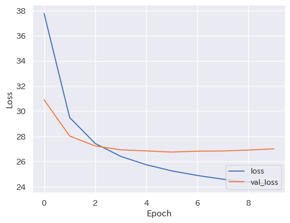
過学習している。
結果
翻訳する
def translator(english_sentence):
    tokenized_english_sentence = english_vectorization_layer([
        "starttoken " + english_sentence + " endtoken"
    ])
    japanese_sentences = ["starttoken"]

    for i in range(JAPANESE_SEQUENCE_LENGTH):
        tokenized_japanese_sentence = japanese_vectorization_layer([
            " ".join(japanese_sentences)
        ])
        decoder_outputs = model(
            (tokenized_english_sentence, tokenized_japanese_sentence)
        )
        decoder_outputs_last_token = tf.argmax(decoder_outputs, axis=-1)[0, i]
        decoder_outputs_last_word = japanese_vocabulary[decoder_outputs_last_token]
        japanese_sentences.append(decoder_outputs_last_word)

        if decoder_outputs_last_word == 'endtoken':
            break

    return "".join(japanese_sentences[1:-1])

print(translator("this is a pen."))
print(translator('i am a student'))
print(translator("i love you."))
print(translator("what are you doing?"))
ペンだ
私は学生だ
愛してる
何をしてるの
attention の可視化
def attentions(english_sentence):
    english_inputs = english_vectorization_layer([
        english_sentence
    ])
    sequences, hidden_state = model.encoder(english_inputs)
    japanese_sentences = ["starttoken"]
    for i in range(JAPANESE_SEQUENCE_LENGTH):
        japanese_inputs = japanese_vectorization_layer([
            " ".join(japanese_sentences)
        ])

        outputs, attentions = model.decoder(japanese_inputs, hidden_state, sequences)
        decoder_outputs_last_token = tf.argmax(outputs, axis=-1)[0, i]

        decoder_outputs_last_word = japanese_vocabulary[decoder_outputs_last_token]
        japanese_sentences.append(decoder_outputs_last_word)

        if decoder_outputs_last_word == 'endtoken':
            break
    return japanese_sentences[1:], attentions[0, :len(english_sentence.split()), :len(japanese_sentences[1:])]

english_sentence = "starttoken there are apple on the table. endtoken"
japanese_sentences, attentions = attentions(english_sentence)
次のコードで可視化する。
# plot attensions

plt.figure(figsize=(16, 6))

ax = sns.heatmap(
    attentions[:len(english_sentence.split())],
    yticklabels=english_sentence.split(),
    xticklabels=japanese_sentences,
    annot=True,
    fmt='.2f',
    cmap='Blues',
)

plt.show()
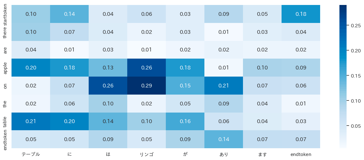
日本語と英語の Attention が可視化できた。
おわりに
チュートリアルではスペイン語と英語は綺麗な Attention を可視化できていたが、日本語と英語ではそこまで綺麗にならなかった。言語の文法上の違いなのか、私のコードが間違ってるのかはわからない。
苦労した点として、きちんと学習が進むように実装する部分が難しかった。特に、RNN の部分は自前で for 文を書くとか、Attention レイヤーは何と何を Attention するのかとかを細かく確認していくのに苦労した。ただ、おかげで RNN と Attention の理解がかなり進んだように思う。意味を理解しながらテンソルを組み合わせてくのが重要。
発展課題として、tensorflow にある Attention を AdditiveAttention 用いて実装を減らすことや、エンコーダーの部分を Bidirectional RNN に置き換えて精度向上を狙うことなどがある。これらは今後挑戦したい。また、2023年 6 月現在だと tensorflow の tutorial は英語版のみアップデートされており、Attention の出力を Decoder の入力に加えない実装となっている。これも挑戦したい。
Discussion