🌻
Hypergeometric vs Binomial Distribution Approximation: A Visualization

2025/07/10に公開
 IntroductionIn the X post, there was the following post from Mr. Osawa.
https://x.com/HirokazuOHSAWA/status/1942942639588073604
Japanese high school mathematics textbooks contain an important statement regarding sampling without replacement:
"Even in the case of sampling without replacement, when the population size is sufficiently large compared to the sample size, the difference between sampling without replacement and sampling with replacement becomes small. Therefore, samples obtained through sampling without replacement can be approximately considered as samples obtained through sampling with replacement, and X₁, X₂, ..., Xₙ can be considered as mutually independent random variables, each following the population distribution."
(Quoted from the textbook of Mathematics B of Shuken Publishing)
While this statement represents a fundamental approximation theory in statistics, it raises the specific question: "To what extent can sampling without replacement be approximately considered as sampling with replacement?" This article aims to provide a quantitative answer to this question through visualization using Julia.

 Theoretical Background
 Relationship between Hypergeometric and Binomial Distributions
Hypergeometric Distribution (sampling without replacement): H(n, K, N) ~ drawing n items without replacement from population N, with K successes

Binomial Distribution (sampling with replacement): B(n, p) ~ n independent trials with success probability p = K/N
When the sampling rate is small (n/N ≪ 1), the hypergeometric distribution can be approximated by the binomial distribution.

 Verification through Visualization
 Basic Comparison Functionusing Plots, Distributions

Plots.default(fontfamily="Hiragino Sans")

# 超幾何分布 vs 二項分布の比較
function compare_hyper_binom(N, K, n)
    p = K/N
    hyper, binom = Hypergeometric(K, N-K, n), Binomial(n, p)
    support = max(0, n+K-N):min(n, K)
    h_pmf, b_pmf = [pdf(hyper, x) for x in support], [pdf(binom, x) for x in support]
    
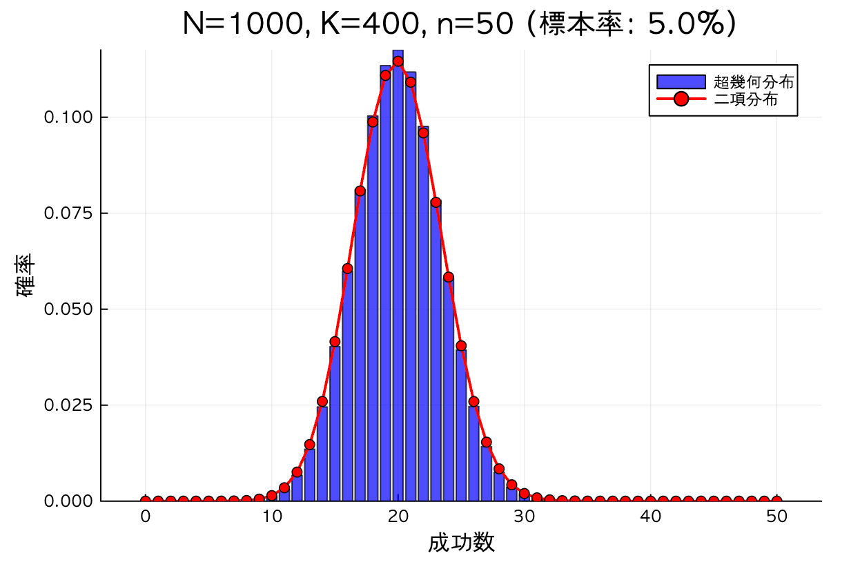
    bar(support, h_pmf, alpha=0.7, label="超幾何分布　　　", color=:blue,
        title="N=$N, K=$K, n=$n (標本率: $(round(100n/N, digits=1))%)")
    plot!(support, b_pmf, marker=:circle, lw=2, ms=4, label="二項分布　　　", color=:red)
    xlabel!("成功数"); ylabel!("確率")
end
compare_hyper_binom(1000, 400, 50)

 1. Effect of Sample RateBy systematically varying the sample rate, we observe how the approximation accuracy changes.
# 標本率効果の比較
function sample_rate_comparison(rates=[0.01, 0.03, 0.05, 0.1, 0.2, 0.3])
    N, K = 1000, 500
    plots = [compare_hyper_binom(N, K, round(Int, N*r)) for r in rates]
    plot(plots..., layout=(2,3), size=(1500, 1000))
end
sample_rate_comparison()
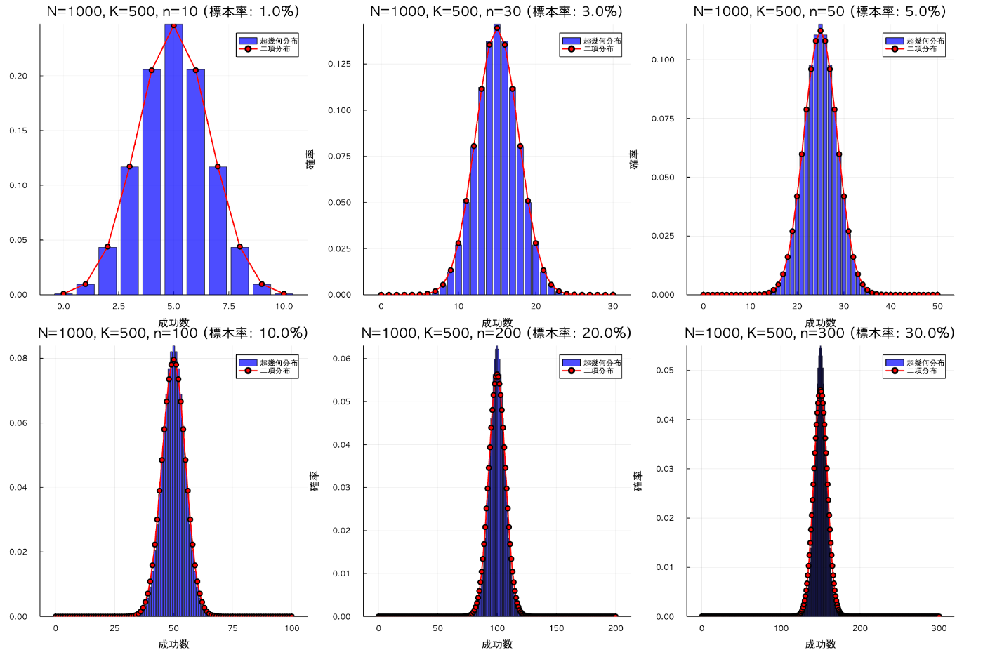
Observations:

Sample rate ≤ 3%: Both distributions are nearly perfectly identical

Sample rate = 5%: Slight differences are visible, but practically sufficient approximation

Sample rate ≥ 10%: Clear differences are observed

 2. Effect of Population SizeWe examine the impact when population size is varied for a fixed sample size.
# 母集団サイズ効果の比較
function population_size_comparison(N_vals=[100, 200, 500, 1000, 2000, 5000])
    n, K_ratio = 50, 0.4
    plots = [compare_hyper_binom(N, round(Int, N*K_ratio), n) for N in N_vals if n ≤ N]
    plot(plots..., layout=(2,3), size=(1500, 1000))
end
population_size_comparison()
Observations:
As population size increases, approximation accuracy improves for the same sample size
For N ≥ 1000, nearly perfect approximation is achieved when n = 50

 3. Quantitative Evaluation: KL DivergenceBeyond visual assessment, we quantify the difference between distributions using KL divergence.
# KLダイバージェンス比較
function kl_comparison(n=50, K_ratio=0.5, N_range=50:50:2000)
    kl_divs, rates = Float64[], Float64[]
    for N in N_range
        n > N && continue
        K = round(Int, N * K_ratio)
        hyper, binom = Hypergeometric(K, N-K, n), Binomial(n, K_ratio)
        support = max(0, n+K-N):min(n, K)
        h_pmf, b_pmf = [pdf(hyper, x) for x in support], [pdf(binom, x) for x in support]
        kl = sum(h_pmf .* log.((h_pmf .+ 1e-10) ./ (b_pmf .+ 1e-10)))
        push!(kl_divs, kl); push!(rates, n/N)
    end
    plot(rates, kl_divs, marker=:circle, lw=2, ms=4, legend=false,
         xlabel="標本率", ylabel="KLダイバージェンス", 
         title="超幾何分布と二項分布の差（KLダイバージェンス）")
    vline!([0.05], ls=:dash, color=:red, lw=2)
end
kl_comparison()
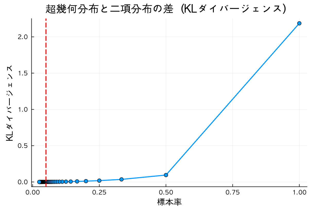
KL Divergence Insights:
KL values decrease exponentially as sample rate decreases
At 5% sample rate, KL values become sufficiently small
Below 1%, KL values approach nearly zero

 Practical Guidelines
 Justification for the 5% RuleThese visualization results confirm the validity of the commonly cited rule in statistics: "If the sample rate is 5% or less, the hypergeometric distribution can be approximated by the binomial distribution."

 Educational Value
Bridge between Theory and Practice: Concrete numerical verification of abstract descriptions in high school mathematics

Parameter Intuition Development: Experience the changes in approximation accuracy under different conditions

Quantitative Thinking Promotion: Objective evaluation using KL divergence as a metric

 ConclusionThe visualization analysis using Julia revealed the following:

Sample rate ≤ 5%: Practically sufficient approximation accuracy

Sample rate ≤ 1%: Nearly perfect approximation

Population size: Larger populations improve approximation accuracy
These results provide concrete criteria for the description in Japanese high school mathematics textbooks: "when the population size is sufficiently large compared to the sample size," contributing to deeper theoretical understanding.

 Complete Codeusing Plots, Distributions

Plots.default(fontfamily="Hiragino Sans")

# 超幾何分布 vs 二項分布の比較
function compare_hyper_binom(N, K, n)
    p = K/N
    hyper, binom = Hypergeometric(K, N-K, n), Binomial(n, p)
    support = max(0, n+K-N):min(n, K)
    h_pmf, b_pmf = [pdf(hyper, x) for x in support], [pdf(binom, x) for x in support]
    
    bar(support, h_pmf, alpha=0.7, label="超幾何分布　　　", color=:blue,
        title="N=$N, K=$K, n=$n (標本率: $(round(100n/N, digits=1))%)")
    plot!(support, b_pmf, marker=:circle, lw=2, ms=4, label="二項分布　　　", color=:red)
    xlabel!("成功数"); ylabel!("確率")
end

# 標本率効果の比較
function sample_rate_comparison(rates=[0.01, 0.03, 0.05, 0.1, 0.2, 0.3])
    N, K = 1000, 500
    plots = [compare_hyper_binom(N, K, round(Int, N*r)) for r in rates]
    plot(plots..., layout=(2,3), size=(1500, 1000))
end

# 母集団サイズ効果の比較
function population_size_comparison(N_vals=[100, 200, 500, 1000, 2000, 5000])
    n, K_ratio = 50, 0.4
    plots = [compare_hyper_binom(N, round(Int, N*K_ratio), n) for N in N_vals if n ≤ N]
    plot(plots..., layout=(2,3), size=(1500, 1000))
end

# KLダイバージェンス比較
function kl_comparison(n=50, K_ratio=0.5, N_range=50:50:2000)
    kl_divs, rates = Float64[], Float64[]
    for N in N_range
        n > N && continue
        K = round(Int, N * K_ratio)
        hyper, binom = Hypergeometric(K, N-K, n), Binomial(n, K_ratio)
        support = max(0, n+K-N):min(n, K)
        h_pmf, b_pmf = [pdf(hyper, x) for x in support], [pdf(binom, x) for x in support]
        kl = sum(h_pmf .* log.((h_pmf .+ 1e-10) ./ (b_pmf .+ 1e-10)))
        push!(kl_divs, kl); push!(rates, n/N)
    end
    plot(rates, kl_divs, marker=:circle, lw=2, ms=4, legend=false,
         xlabel="標本率", ylabel="KLダイバージェンス", 
         title="超幾何分布と二項分布の差（KLダイバージェンス）")
    vline!([0.05], ls=:dash, color=:red, lw=2)
end

# 全体デモ
function demo()
    println("1. 標本率の効果:"); display(sample_rate_comparison())
    println("2. 母集団サイズの効果:"); display(population_size_comparison()) 
    println("3. KLダイバージェンス:"); display(kl_comparison())
end

# 使用例
println("使用方法: demo(), sample_rate_comparison(), population_size_comparison(), kl_comparison()")
println("個別比較: compare_hyper_binom(1000, 400, 50)")

 Key FindingsThe visualization confirms that:

The 5% rule is scientifically justified through both visual and quantitative analysis

Population size matters: Larger populations allow for better approximations even with the same sample size

KL divergence provides objective measurement: The exponential decrease in KL values as sample rate decreases gives mathematical support to the approximation rule
This analysis bridges the gap between theoretical statements in textbooks and practical understanding through computational verification.