「数学ガール　リーマン予想」を読みました

はじめに

2025年8月7日に結城浩さんの著書　「数学ガール　リーマン予想」が発売されました。17年に渡り出版された「数学ガール」シリーズの完結編とのことです。私自身も読ませていただき，学校の生徒にもレコメンドさせていただきました。

https://www.sbcr.jp/product/4815628727/

せっかくなので，第1章から第10章の中で出てきたものをJulia言語を使って表現してみました。
あたらめて，結城浩さんに感謝を込めて，作品をありがとうございました。

第1章　素数定理

$$\frac{\pi(x)}x \sim \frac1{\log x}$$

using Primes

function sosuu_optimized(n)
    if n <= 1000
        # 関数内で素数リストを生成（初回のみ計算される）
        primes_list = primes(1000)
        return count(p -> p <= n, primes_list) / n
    else
        samples = 10^4
        k = 0
        for _ = 1:samples
            k += rand(1:n) |> isprime
        end
        return k / samples
    end
end

X = 1:1000
Y = sosuu_optimized.(X)
using Plots
plot(X, Y)
plot!(x->1/log(x),ylim=(0,0.7))

using Primes

function sosuu_exact(n)
    return length(primes(n)) / n
end

# 使用例
X = 1:1000
Y = sosuu_exact.(X)
using Plots
plot(X, Y)
plot!(x->1/log(x),ylim=(0,0.7))

第2章　オイラー積

$$\prod_{素数 p} \frac{1}{1-\frac1{p^s}}= \sum_{自然数 n} \frac{1}{n^s}$$

using Plots, Primes

function euler_zeta_comparison(s=2.0)
    # 級数側: ∑(1/n^s)
    series(n) = sum(1/k^s for k in 1:n)
    
    # オイラー積側: ∏(1/(1-1/p^s))
    product(max_p) = prod(1/(1-1/p^s) for p in primes(max_p))
    
    # データ生成
    n_vals = 10:10:1000
    p_vals = 2:50
    
    series_vals = [series(n) for n in n_vals]
    product_vals = [product(p) for p in p_vals]
    
    # 別々のプロット作成
    p_series = plot(n_vals, series_vals, label="Series ∑1/n^s", lw=2, color=:blue,
                   title="Series (s=$s)", xlabel="Terms", ylabel="ζ($s)")
    
    p_product = plot(length.(primes.(p_vals)), product_vals, label="Euler Product ∏1/(1-1/p^s)", 
                    lw=2, color=:red, title="Euler Product (s=$s)", 
                    xlabel="Number of primes", ylabel="ζ($s)")
    
    # 理論値追加 (s=2の場合)
    if s ≈ 2
        hline!(p_series, [π^2/6], label="π²/6", color=:green, lw=2)
        hline!(p_product, [π^2/6], label="π²/6", color=:green, lw=2)
    end
    
    return plot(p_series, p_product, layout=(1,2))
end

# 複数のsで比較 (横に2列配置)
plots = [euler_zeta_comparison(s) for s in [1.5, 2.0, 3.0, 4.0]]
plot(plots..., layout=(4,1), size=(800,1000))

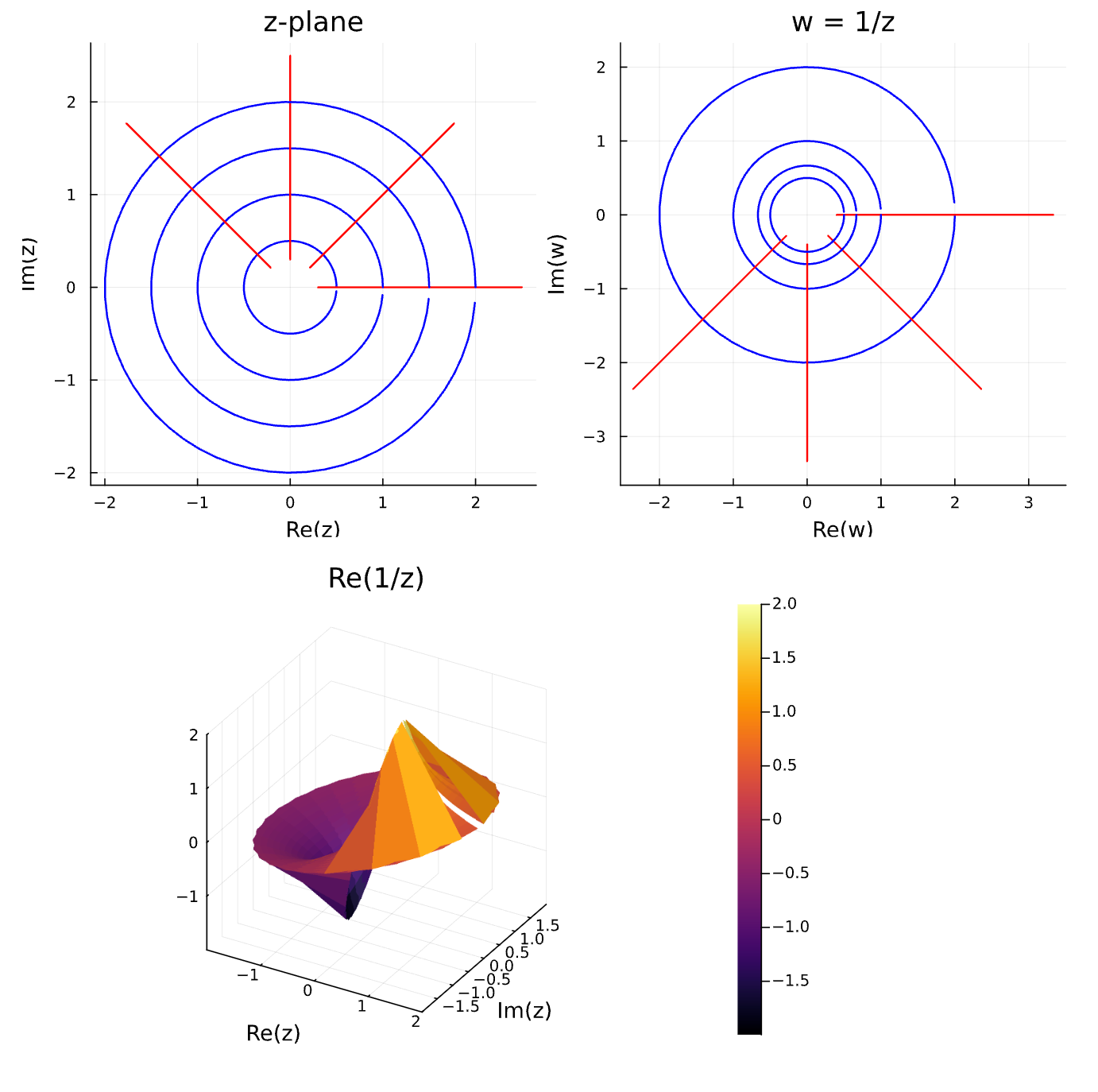
第3章　無限遠点で待ち合わせ

$$w = \frac1z$$

using Plots

# w = 1/z の可視化
function visualize_inversion()
    # 同心円と放射線
    θ = 0:0.1:2π
    circles = [[r*exp(1im*t) for t in θ] for r in [0.5, 1.0, 1.5, 2.0]]
    lines = [[r*exp(1im*angle) for r in 0.3:0.1:2.5] for angle in 0:π/4:2π-π/4]
    
    # 変換 w = 1/z
    circles_w = [1 ./ circle for circle in circles]
    lines_w = [1 ./ line for line in lines]
    
    # プロット
    p1 = plot(title="z-plane", xlabel="Re(z)", ylabel="Im(z)", aspect_ratio=:equal, legend=false)
    for i in 1:4
        plot!(p1, real.(circles[i]), imag.(circles[i]), color=:blue, lw=1.5)
        plot!(p1, real.(lines[i]), imag.(lines[i]), color=:red, lw=1.5)
    end
    
    p2 = plot(title="w = 1/z", xlabel="Re(w)", ylabel="Im(w)", aspect_ratio=:equal, legend=false)
    for i in 1:4
        plot!(p2, real.(circles_w[i]), imag.(circles_w[i]), color=:blue, lw=1.5)
        plot!(p2, real.(lines_w[i]), imag.(lines_w[i]), color=:red, lw=1.5)
    end
    
    plot(p1, p2, layout=(1,2), size=(800,400))
end

# リーマン面 3D
function riemann_surface()
    r = 0.5:0.1:2
    θ = 0:0.2:2π
    
    Z = [ri*exp(1im*ti) for ti in θ, ri in r]
    W = 1 ./ Z
    
    X, Y = real.(Z), imag.(Z)
    surface(X, Y, real.(W), title="Re(1/z)", xlabel="Re(z)", ylabel="Im(z)")
end

# 実行
display(visualize_inversion())
display(riemann_surface())

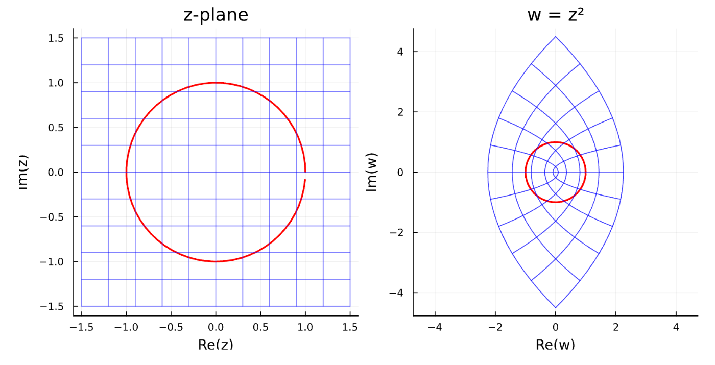
第4章　複素関数の探険

$$w = z^2$$

using Plots

# 複素変換 w = z² の可視化
function visualize_complex_transform()
    # 単位円と格子線
    θ = 0:0.1:2π
    circle = [exp(1im*t) for t in θ]
    
    # 格子線作成
    lines = []
    for i in -1.5:0.3:1.5
        push!(lines, [complex(i, y) for y in -1.5:0.1:1.5])  # 垂直線
        push!(lines, [complex(x, i) for x in -1.5:0.1:1.5])  # 水平線
    end
    
    # 変換適用
    circle_w = circle.^2
    lines_w = [line.^2 for line in lines]
    
    # プロット
    p1 = plot(title="z-plane", xlabel="Re(z)", ylabel="Im(z)", 
              aspect_ratio=:equal, legend=false)
    plot!(p1, real.(circle), imag.(circle), color=:red, lw=2, label="Unit circle")
    for line in lines
        plot!(p1, real.(line), imag.(line), color=:blue, alpha=0.5)
    end
    
    p2 = plot(title="w = z²", xlabel="Re(w)", ylabel="Im(w)", 
              aspect_ratio=:equal, legend=false)
    plot!(p2, real.(circle_w), imag.(circle_w), color=:red, lw=2, label="Transformed")
    for line in lines_w
        plot!(p2, real.(line), imag.(line), color=:blue, alpha=0.5)
    end
    
    plot(p1, p2, layout=(1,2), size=(800,400))
end

# 実行
visualize_complex_transform()

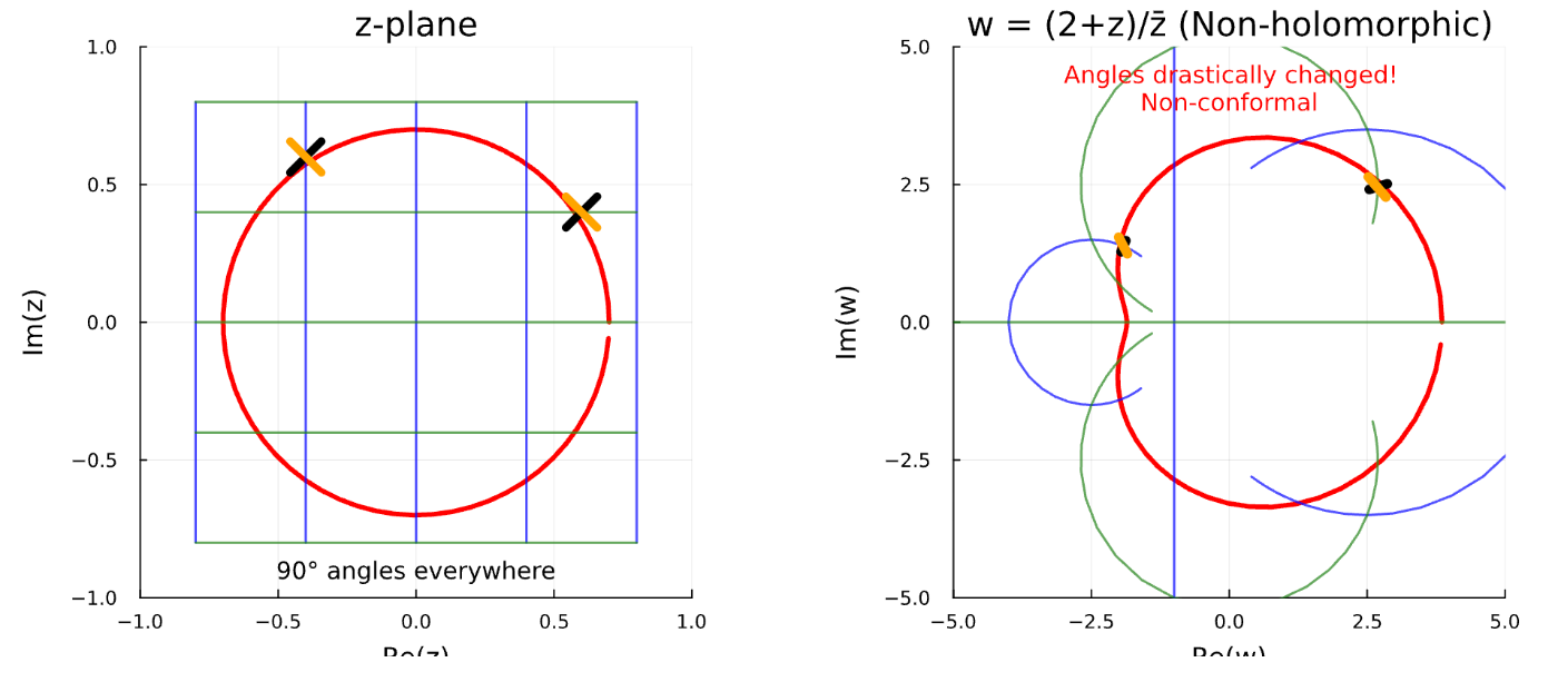
第5章　複素関数の微分

$$w = \frac{2+z}{\overline{z}}$$

using Plots

# 複素変換 w = (2+z)/z̄ の可視化（非正則で角度も変わる例）
function visualize_complex_transform()
    # 単位円と格子線
    θ = 0:0.1:2π
    circle = [0.7*exp(1im*t) for t in θ]
    
    # 等角性を調べるための直交する曲線
    orthogonal_lines = []
    # 垂直線
    for x in [-0.8, -0.4, 0, 0.4, 0.8]
        push!(orthogonal_lines, [complex(x, y) for y in -0.8:0.05:0.8])
    end
    # 水平線
    for y in [-0.8, -0.4, 0, 0.4, 0.8]
        push!(orthogonal_lines, [complex(x, y) for x in -0.8:0.05:0.8])
    end
    
    # 変換適用 w = (2+z)/z̄ (非正則関数)
    circle_w = (2 .+ circle) ./ conj.(circle)
    orthogonal_lines_w = [(2 .+ line) ./ conj.(line) for line in orthogonal_lines]
    
    # 角度変化を示すテスト点で直交する線分（角度変化が大きい位置を選択）
    test_points = [0.6+0.4im, -0.4+0.6im]  # 実軸・虚軸から離れた位置
    
    # プロット
    p1 = plot(title="z-plane", xlabel="Re(z)", ylabel="Im(z)", 
              aspect_ratio=:equal, legend=false, xlims=(-1, 1), ylims=(-1, 1))
    plot!(p1, real.(circle), imag.(circle), color=:red, lw=3)
    
    # 直交格子
    for i in 1:5
        plot!(p1, real.(orthogonal_lines[i]), imag.(orthogonal_lines[i]), 
              color=:blue, lw=1.5, alpha=0.7)
    end
    for i in 6:10
        plot!(p1, real.(orthogonal_lines[i]), imag.(orthogonal_lines[i]), 
              color=:green, lw=1.5, alpha=0.7)
    end
    
    # 各テスト点で90度の角を表示（斜めの方向で）
    for pt in test_points
        # 45度と135度方向の線分（より角度変化が見えやすい）
        dir1 = exp(1im * π/4)    # 45度方向
        dir2 = exp(1im * 3π/4)   # 135度方向
        line1 = [pt - 0.08*dir1, pt + 0.08*dir1]
        line2 = [pt - 0.08*dir2, pt + 0.08*dir2]
        plot!(p1, real.(line1), imag.(line1), color=:black, lw=5)
        plot!(p1, real.(line2), imag.(line2), color=:orange, lw=5)
    end
    
    p2 = plot(title="w = (2+z)/z̄ (Non-holomorphic)", xlabel="Re(w)", ylabel="Im(w)", 
              aspect_ratio=:equal, legend=false, xlims=(-5, 5), ylims=(-5, 5))
    plot!(p2, real.(circle_w), imag.(circle_w), color=:red, lw=3)
    
    # 変換後の格子（見やすくするため一部のみ表示）
    for i in [2, 3, 4]  # 中央付近の線のみ
        line_w = orthogonal_lines_w[i]
        # 極端に大きな値を除外
        valid_indices = findall(z -> abs(z) < 10, line_w)
        if length(valid_indices) > 5
            plot!(p2, real.(line_w[valid_indices]), imag.(line_w[valid_indices]), 
                  color=:blue, lw=1.5, alpha=0.7)
        end
    end
    for i in [7, 8, 9]  # 中央付近の線のみ
        line_w = orthogonal_lines_w[i]
        valid_indices = findall(z -> abs(z) < 10, line_w)
        if length(valid_indices) > 5
            plot!(p2, real.(line_w[valid_indices]), imag.(line_w[valid_indices]), 
                  color=:green, lw=1.5, alpha=0.7)
        end
    end
    
    # 変換後の各点での角度
    for pt in test_points
        if abs(pt) > 0.2
            delta = 0.04
            dir1 = exp(1im * π/4)
            dir2 = exp(1im * 3π/4)
            
            pt1, pt2 = pt + delta*dir1, pt - delta*dir1
            pt3, pt4 = pt + delta*dir2, pt - delta*dir2
            
            if all(abs.([pt1, pt2, pt3, pt4]) .> 0.1)
                line1_w = [(2 + pt1)/conj(pt1), (2 + pt2)/conj(pt2)]
                line2_w = [(2 + pt3)/conj(pt3), (2 + pt4)/conj(pt4)]
                
                # 結果が表示範囲内の場合のみプロット
                if all(abs.(vcat(line1_w, line2_w)) .< 8)
                    plot!(p2, real.(line1_w), imag.(line1_w), color=:black, lw=6)
                    plot!(p2, real.(line2_w), imag.(line2_w), color=:orange, lw=6)
                end
            end
        end
    end
    
    # 説明テキスト
    annotate!(p1, 0, -0.9, text("90° angles everywhere", 10, :black))
    annotate!(p2, 0, 4.5, text("Angles drastically changed!", 10, :red))
    annotate!(p2, 0, 4.0, text("Non-conformal", 10, :red))
    
    plot(p1, p2, layout=(1,2), size=(1000,400))
end

# 実行
visualize_complex_transform()

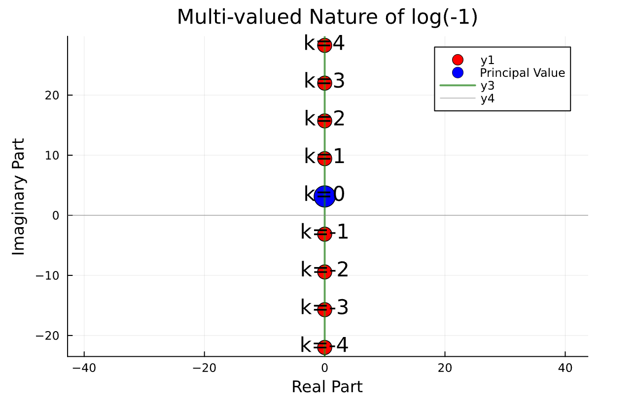
第6章　log(-1)の螺旋階段

$$\log(-1) = (2k+1)\pi i , k \in \mathbb{Z}$$

using Plots

# log(-1) = i(π + 2πk) の可視化
k_values = -4:4
log_values = [im * (π + 2π * k) for k in k_values]

# 複素平面にプロット
real_parts = real.(log_values)
imag_parts = imag.(log_values)

scatter(real_parts, imag_parts,
        title="Multi-valued Nature of log(-1)",
        xlabel="Real Part", ylabel="Imaginary Part",
        markersize=8, color=:red,
        grid=true, aspect_ratio=:equal)

# 主値（k=0）を強調
scatter!([0], [π], markersize=12, color=:blue, label="Principal Value")

# 各点にラベル
for (i, k) in enumerate(k_values)
    annotate!(0, imag_parts[i] + 0.5, "k=$k")
end

# 軸を強調
vline!([0], color=:green, linewidth=2, alpha=0.7)
hline!([0], color=:gray, alpha=0.5)

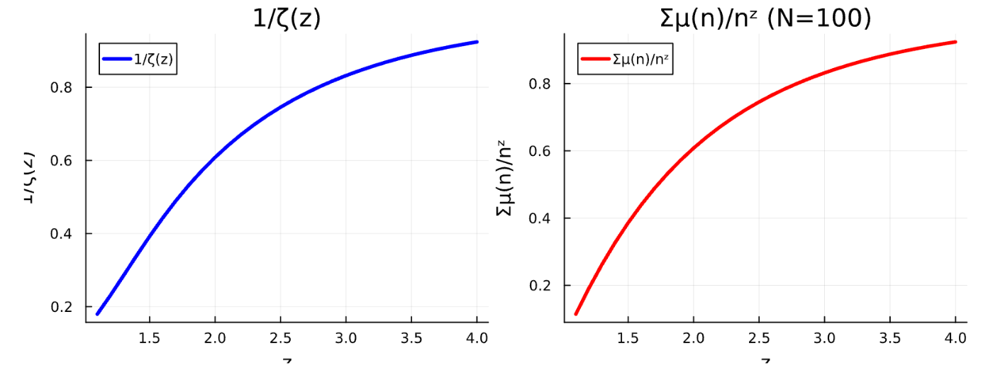
第7章　ゼータ関数とメビウス関数

$$\frac1{\zeta(z)}=\sum_{n=1}^\infty \frac{\mu(n)}{n^z}$$

using Plots

# メビウス関数
mobius(n) = begin
    factors = []
    temp, d = n, 2
    while d * d <= temp
        while temp % d == 0
            push!(factors, d)
            temp ÷= d
        end
        d += 1
    end
    temp > 1 && push!(factors, temp)
    length(factors) != length(unique(factors)) ? 0 : (-1)^length(factors)
end

# 関数定義
zeta(z) = sum(1.0/n^z for n in 1:1000)
mobius_sum(z, N) = sum(mobius(n) / n^z for n in 1:N)

# z の範囲
z = 1.1:0.1:4.0

# 左側：1/ζ(z)
p1 = plot(z, 1 ./zeta.(z), linewidth=3, color=:blue, 
         title="1/ζ(z)", xlabel="z", ylabel="1/ζ(z)", 
         label="1/ζ(z)")

# 右側：Σμ(n)/n^z (N=100)
p2 = plot(z, [mobius_sum(zi, 100) for zi in z], linewidth=3, color=:red,
         title="Σμ(n)/nᶻ (N=100)", xlabel="z", ylabel="Σμ(n)/nᶻ",
         label="Σμ(n)/nᶻ")

# 左右に並べて表示
plot(p1, p2, layout=(1,2), size=(800,300))

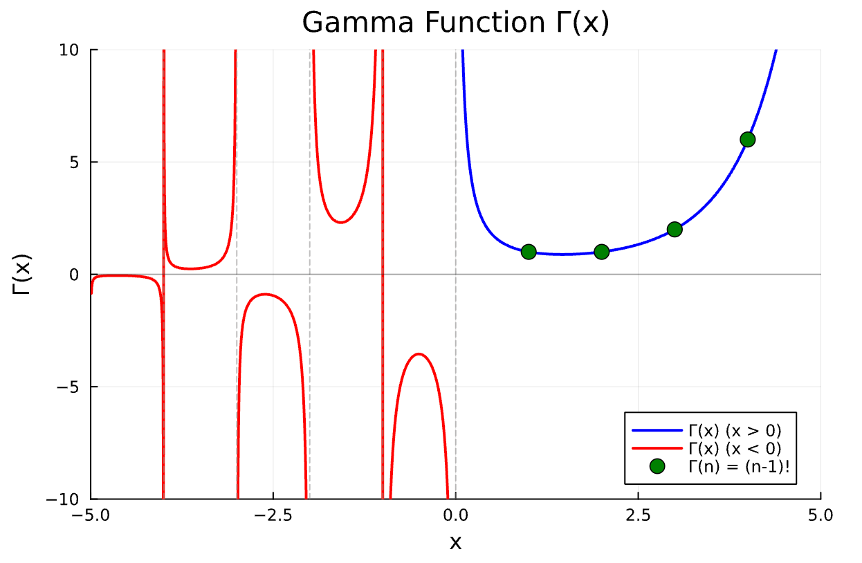
第8章　驚きのガンマ関数

$$\Gamma(x) =\int_0^\infty e^{-t} t^{x-1} dt$$

using Plots
using SpecialFunctions

# ガンマ関数のプロット（負の範囲も含む）
x_pos = range(0.01, 5.0, length=1000)
x_neg = range(-4.99, -0.01, length=1000)

# 正の範囲
y_pos = gamma.(x_pos)

# 負の範囲（極での発散を避けるため区間を分割）
function safe_gamma(x)
    # 負の整数近傍で発散するのでNaNを返す
    if abs(x - round(x)) < 0.001 && x < 0
        return NaN
    else
        return gamma(x)
    end
end

y_neg = safe_gamma.(x_neg)

# プロット
plot(x_pos, y_pos, color=:blue, linewidth=2, label="Γ(x) (x > 0)",
     ylims=(-10, 10), xlims=(-5, 5),
     title="Gamma Function Γ(x)", xlabel="x", ylabel="Γ(x)",
     grid=true)

plot!(x_neg, y_neg, color=:red, linewidth=2, label="Γ(x) (x < 0)")

# 特別な値をマーク
scatter!([1, 2, 3, 4], [1, 1, 2, 6], color=:green, markersize=6, 
         label="Γ(n) = (n-1)!")

# 極（負の整数）を垂直線で示す
for n in -4:0
    vline!([n], color=:gray, linestyle=:dash, alpha=0.5, label="")
end

# 水平線
hline!([0], color=:black, alpha=0.3, label="")

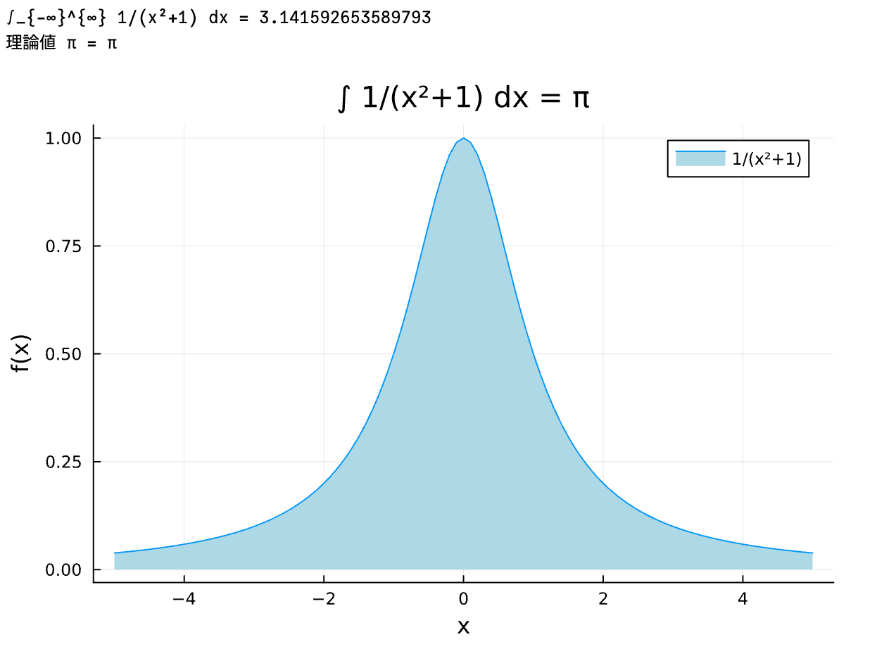
第9章　複素積分ひとめぐり

$$\int_{-\infty}^\infty \frac1{x^2+1} dx = \pi$$

using QuadGK, Plots

# 積分計算
f(x) = 1/(x^2 + 1)
result, _ = quadgk(f, -Inf, Inf)

println("∫_{-∞}^{∞} 1/(x²+1) dx = $result")
println("理論値 π = $π")

# プロット
x = -5:0.1:5
y = f.(x)
plot(x, y, fill=(0, :lightblue), title="∫ 1/(x²+1) dx = π", 
     xlabel="x", ylabel="f(x)", label="1/(x²+1)")

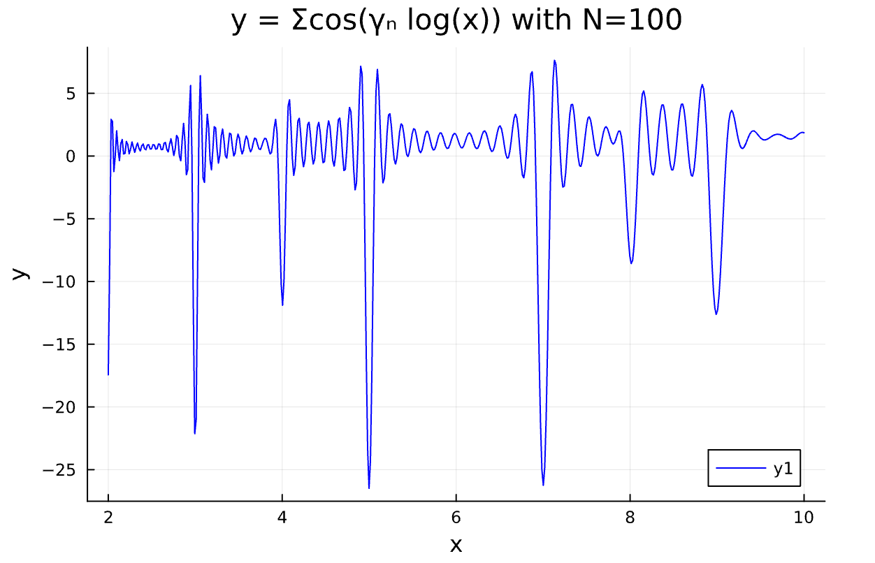
第10章　リーマン予想

$$y = \sum_{n=1}^{100} \cos(\Im(p_n)\log x)$$

• $p_n$のデータベースは下記のサイトより

https://www.plouffe.fr/simon/constants/zeta100.html

using Plots

# リーマン零点（虚部）- Odlyzkoのデータベースから最初の100個
γ = [
    14.134725141734693790457251983562470270784257115699243175685567460149,
    21.022039638771549926284795318956902777334340524902781754629520403587,
    25.010857580145688763213790992562821818659549672557996672496542006745,
    30.424876125859513210311897530584091320181560023715440180962146036993,
    32.935061587739189690662368964074903488812715603517039009280003440784,
    37.586178158825671257217763480705332821405597350830793218333001113622,
    40.918719012147495187398126914633254395726165962777279536161303667253,
    43.327073280914999519496122165406805782645668371836871446878893685521,
    48.005150881167159727942472749427516041686844001144425117775312519814,
    49.773832477672302181916784678563724057723178299676662100781955750433,
    52.970321477714460644147296608880990063825017888821224779900748140317,
    56.446247697063394804367759476706127552782264471716631845450969843958,
    59.347044002602353079653648674992219031098772806466669698122451754746,
    60.831778524609809844259901824524003802910090451219178257101348824808,
    65.112544048081606660875054253183705029348149295166722405966501086675,
    67.079810529494173714478828896522216770107144951745558874196669551694,
    69.546401711173979252926857526554738443012474209602510157324539999663,
    72.067157674481907582522107969826168390480906621456697086683306151488,
    75.704690699083933168326916762030345922811903530697400301647775301574,
    77.144840068874805372682664856304637015796032449234461041765231453151,
    79.337375020249367922763592877116228190613246743120030878438720497101,
    82.910380854086030183164837494770609497508880593782149146571306283235,
    84.735492980517050105735311206827741417106627934240818702735529689045,
    87.425274613125229406531667850919213252171886401269028186455557938439,
    88.809111207634465423682348079509378395444893409818675042199871618814,
    92.491899270558484296259725241810684878721794027730646175096750489181,
    94.651344040519886966597925815208153937728027015654852019592474274513,
    95.870634228245309758741029219246781695256461224987998420529281651651,
    98.831194218193692233324420138622327820658039063428196102819321727565,
    101.31785100573139122878544794029230890633286638430089479992831871523,
    103.72553804047833941639840810869528083448117306949576451988516579403,
    105.44662305232609449367083241411180899728275392853513848056944711418,
    107.16861118427640751512335196308619121347670788140476527926471042155,
    111.02953554316967452465645030994435041534596839007305684619079476550,
    111.87465917699263708561207871677059496031174987338587381661941961969,
    114.32022091545271276589093727619107980991765772382989228772843104130,
    116.22668032085755438216080431206475512732985123238322028386264231147,
    118.79078286597621732297913970269982434730621059280938278419371651419,
    121.37012500242064591894553297049992272300131063172874230257513263573,
    122.94682929355258820081746033077001649621438987386351721195003491528,
    124.25681855434576718473200796612992444157353877469356114035507691395,
    127.51668387959649512427932376690607626808830988155498248279977930068,
    129.57870419995605098576803390617997360864095326465943103047083999886,
    131.08768853093265672356637246150134905920354750297504538313992440777,
    133.49773720299758645013049204264060766497417494390467501510225885516,
    134.75650975337387133132606415716973617839606861364716441697609317354,
    138.11604205453344320019155519028244785983527462414623568534482856865,
    139.73620895212138895045004652338246084679005256538260308137013541090,
    141.12370740402112376194035381847535509030066087974762003210466509596,
    143.11184580762063273940512386891392996623310243035463254859852295728,
    146.00098248676551854740250759642468242897574123309580363697688496658,
    147.42276534255960204952118501043150616877277525047683060101046081273,
    150.05352042078488035143246723695937062303732155952820044842911127506,
    150.92525761224146676185252467830562760242677047299671770031135495336,
    153.02469381119889619825654425518544650859043490414550667519976756379,
    156.11290929423786756975018931016919474653530850094292080385607815839,
    157.59759181759405988753050315849876573072389951914173353824961760978,
    158.84998817142049872417499477554027141433508304942696625772418341154,
    161.18896413759602751943734412936955436491579032747546657918809379411,
    163.03070968718198724331103900068799489696446141647768311520959169590,
    165.53706918790041883003891935487479732836725174506860447895315460558,
    167.18443997817451344095775624621037873646076924261676736110699343540,
    169.09451541556882148950587118143183479666764858044162508738214912188,
    169.91197647941169896669984359582179228839443712534137301854144160780,
    173.41153651959155295984611864934559525415606606342011793368228539153,
    174.75419152336572581337876245586691793875571762057166344561154743789,
    176.44143429771041888889264105786093352811849710880971534761261578625,
    178.37740777609997728583093541418442618313236146127250370148904080374,
    179.91648402025699613934003661205123745368760755301840654130067065381,
    182.20707848436646191540703722698779869079745777823990876663006454018,
    184.87446784838750880096064661723425841335102291195066777317864468070,
    185.59878367770747146652770426839264661293471764951328308891979623038,
    187.22892258350185199164154058613124301681073460399031915146420316373,
    189.41615865601693708485228909984532449135710302319335435541994217710,
    192.02665636071378654728363142558343010583992029797709691628912343221,
    193.07972660384570404740220579437605460402061581054886013850435583088,
    195.26539667952923532146318781486225092690505245228692406011097663218,
    196.87648184095831694862226391469620773574602869194221548282317318163,
    198.01530967625191242491991870220886715506269543857099672153480159423,
    201.26475194370378873301613342754817322240286363918673408063271979951,
    202.49359451414053427768666063786431582102024489942005390906915428511,
    204.18967180310455433071643838631368513653452922874190735095968021739,
    205.39469720216328602521237939069309092372291477204840700213409541714,
    207.90625888780620986150196790775364426865940376888399985865752750992,
    209.57650971685625985283564428988675217539078318132616246897745334620,
    211.69086259536530756390748673071929425339403098293564373621001482077,
    213.34791935971266619063912202107260882189718327663306905985370458536,
    214.54704478349142322294420107259069104559988805308307640008161991904,
    216.16953850826370026586956335449812857545371427416411097637615056594,
    219.06759634902137898567725659043724124514918292701135137355787499323,
    220.71491883931400336911559263390633965676114507766196570161193204082,
    221.43070555469333873209747511927607795022233107731990937941995151378,
    224.00700025460433521172887552850489535608598994959552976295036068233,
    224.98332466958228750378252368052865677209005448558742698847775254720,
    227.42144427967929131046143616065963996396914832197662836489382008238,
    229.33741330552534810776008330605574008275234138781851753263649248435,
    231.25018870049916477380618677001037260670849584312337140680603034414,
    231.98723525318024860377166853919786220541983399456249648472682389683,
    233.69340417890830064070449473256978817953722775456583636301480873894,
    236.52422966581620580247550795566297868952949521218912370091896098781
]

# 級数計算
f(x) = sum(cos(γₙ * log(x)) for γₙ in γ)


# プロット
x = range(2, 10, length=500)
plot(x, f.(x), title="y = Σcos(γₙ log(x)) with N=100", xlabel="x", ylabel="y", 
     linewidth=1, color=:blue)