GIS × Python Tutorial 6.3 ~ 地上分解能の決め方とRGB画像の作成 ~
この記事は「GIS × Python Tutorial」の関連記事です。
はじめに
前回の記事では CSF(Cloth Simulation Filter) による点群分類と DTM(Digital Terrain Model) の作成を行いました。
今回は DTM の後処理を行う予定でしたが、以前の記事では地上分解能をさらっと適当に決めていたり、RGB画像を登場させていたので、今回は先にその部分についてを解説していきます。
-
オルソ画像とは
-
点群データを画像化する為の準備
-
RGB 画像の作成
-
Raster の出力
-
Intensity を見てみる
-
バンド合成で遊ぶ
今回使用するデータ
今回は Session6 の記事で作成した '.las' を使用します。元々はオープンナガサキからダウンロードした点群データです。
インポート
from IPython.display import Image
import japanize_matplotlib
from matplotlib import pyplot as plt
from matplotlib.spines import Spine
import matplotlib.patches as mpatches
from mpl_toolkits.axes_grid1.inset_locator import inset_axes
import numpy as np
import pdal
import pyproj
import rasterio
import rasterio.mask
import rasterio.plot
import shapely
from shapely.plotting import plot_polygon
japanize_matplotlib.japanize()


IN_FILE = r'../datasets/01ID7913_proj.las'

# 長崎県のEPSGコード
IN_EPSG = 'EPSG:6669'
proj_crs = pyproj.CRS(IN_EPSG)
IN_SRS = proj_crs.to_wkt(pretty=True)
1. オルソ画像とは
オルソ画像 とは上空から撮影した画像を正射変換し、真上から見たような傾きの無い、正しい大きさと位置に表示される様に変換した画像の事です。
上空の遠く離れた場所から大きな範囲を撮影した画像は、画像の端に行くほどに、写真に映る物体が大きく斜めに傾いて映っています。
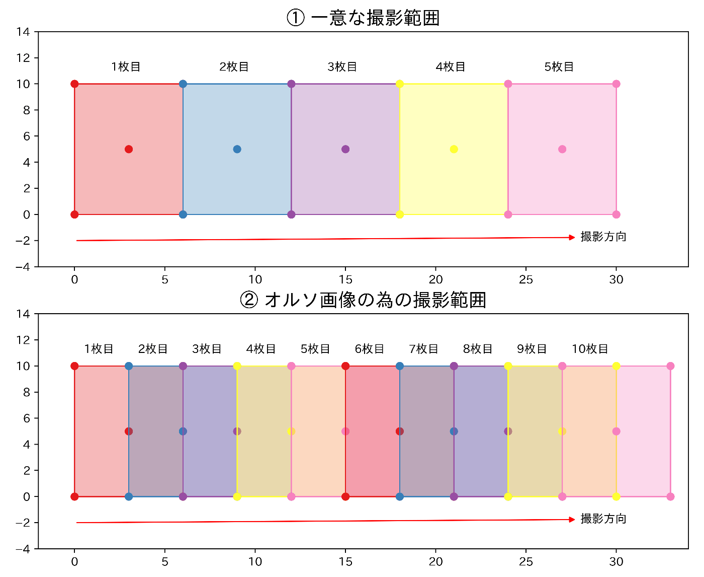
オルソ画像を作成する場合の撮影は、以下の①の様に一意な範囲を撮影するのではなく、②の様に同じ場所が複数の写真に映るように撮影します。その画像を合成する事でオルソ画像を作成します。
進行方向に重なっている範囲を'オーバーラップ率'、折り返しなどで別なコースの写真と重なっている範囲を'サイドラップ率'と呼びます。
今回は点群データから画像を作成するだけなので、オルソ画像ではありませんが、見た目は似たものになるので...
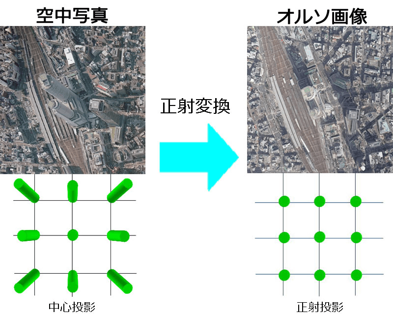
画像引用:国土地理院
2. 点群データを画像化する為の準備
PDAL で点群データから RGB 画像を作成するのは非常に簡単です。但しこれは点群データに RGB の情報が入力されている場合に限ります。
以前の記事でも見ましたが、まずは「点群データ(.las)にどんな情報が入力されているのか」を確かめてみましょう。
以前の記事では、Dict の中に Pipeline の処理を書いて、JSON 文字列化して処理を実行しましたが今回は別な書き方をしてみます。
2-1. 有用な要素の確認
点群データの中から使用できそうな要素を確認します。要素の種類自体は多くありますが、実際に使用可能な要素は多くありません。pandas.DataFrame の形に変換し、不要な列を削除します。
readers = pdal.Reader.las(r'../datasets/01ID7913_proj.las')
pipeline = readers.pipeline()
pipeline.execute()
df = pipeline.get_dataframe(0)


del_cols = []
for col in df.columns:
    if len(df[col].unique()) == 1:
        del_cols.append(col)

df.drop(del_cols, axis=1).describe()
                  X             Y             Z     Intensity           Red  \
count  6.684581e+06  6.684581e+06  6.684581e+06  6.684581e+06  6.684581e+06
mean  -3.484883e+03  3.786842e+04  3.154098e+02  1.676435e+02  2.039356e+04
std    2.881643e+02  2.167067e+02  6.870297e+01  6.171454e+01  8.347706e+03
min   -4.000000e+03  3.750000e+04  1.428500e+02  0.000000e+00  5.140000e+02
25%   -3.731850e+03  3.768077e+04  2.672600e+02  1.340000e+02  1.310700e+04
50%   -3.475220e+03  3.786558e+04  2.959000e+02  1.790000e+02  1.927500e+04
75%   -3.233750e+03  3.805521e+04  3.566900e+02  2.120000e+02  2.698500e+04
max   -3.000000e+03  3.825000e+04  5.196200e+02  2.550000e+02  6.553500e+04

              Green          Blue
count  6.684581e+06  6.684581e+06
mean   2.492939e+04  2.461110e+04
std    6.574588e+03  5.020807e+03
min    7.196000e+03  1.799000e+03
25%    1.927500e+04  2.081700e+04
50%    2.415800e+04  2.364400e+04
75%    2.981200e+04  2.775600e+04
max    6.553500e+04  6.553500e+04
画像の作成に使用出来そうな値は、「Intensity(反射強度)」「Red」「Green」「Blue」 の4種類ですね。
2-2. 地上分解能の大きさを決める
まずはパラメーターを設定します。地上分解能とはセルの大きさを現実世界に当て嵌めた時の、1セルの大きさの事です。このセルの範囲に含まれる、点群の要素を計算して画像を作成するので、この大きさを考えるのは重要なタスクです。
国土地理院の公開している「UAV搭載型レーザースキャナを用いた公共測量マニュアル(案)」では以下の様に書かれています。
準則の航空レーザ測量では、グリッドデータを作成する際に、点群が取得できない格子の割合を欠測率として定めている。準則第435条では『欠測率=(欠測格子数/格子数)×100)』と定め、格子間隔が1mを超えるグリッドデータを作成する場合の欠測率は10%以下、1m以下の場合は15%以下を標準としている。
今回作成するデータは RGB 画像ですが、欠測率を調べてみましょう。この記事を書く際に、最初は自分で shapely.Polygon で MeshGrid を作成し、空間検索と集計処理をして欠測率を求めましたが、計算に結構な時間が掛かりました。なので今回は PDAL を使用して、各セルに含まれる点群の数を数えます。
PDAL を使用して各セルに含まれる点群を数える為に、点群データを画像化する際の計算でセル内の計測点数を数える事にします。以前は PDAL を使用する際、辞書型のオブジェクトに Pipeline の処理内容を書きましたが、今回は別な書き方で書いてみましょう。
COUNT_PATH = IN_FILE.replace('proj.las', 'COUNT.tif')
RESOLUTION = 0.5

# データの読み込み
readers = readers = pdal.Reader.las(IN_FILE)

# グリッド内の点群を数え画像化して出力する
writers = (
    pdal
    .Writer(
        type='writers.gdal',
        filename=COUNT_PATH,
        data_type='uint16',
        resolution=RESOLUTION,
        dimension='Z',
        output_type='count',
        nodata=0,
        default_srs=IN_SRS,
        gdaldriver='GTiff'
    )
)
# Pipelineの作成と実行
pipeline = readers  | writers
pipeline.execute()
次は出力した Raster を読み込んで欠測率を確認してみましょう。Raster の入出力や加工には rasterio というライブラリーを使用します。GDAL の方が有名かもしれませんが、python で扱うのであれば rasterio の方が簡単で、ドキュメントも読みやすいので、おススメです。
with rasterio.open(COUNT_PATH) as dst:
    count_img = dst.read(1)


def formatter(val):
    return '{:,}'.format(val)


count_ary_1d = count_img.flatten()
count_cell = len(count_ary_1d)
count_loss = len(count_ary_1d[count_ary_1d == 0])
loss_rate = round(count_loss / count_cell * 100, 2)

print(
f"""
shape      : {count_img.shape}
格子数     : {formatter(count_cell)}
欠測格子数 : {formatter(count_loss)}
欠測率     : {loss_rate} %
最大計測数 : {np.max(count_ary_1d)}
最小計測数 : {np.min(count_ary_1d)}
平均計測数 : {round(np.mean(count_ary_1d), 2)}
shape      : (1501, 2001)
格子数     : 3,003,501
欠測格子数 : 1,175
欠測率     : 0.04 %
最大計測数 : 154
最小計測数 : 0
平均計測数 : 13.96
平均値と最大値が離れているので、可視化しようとすると、外れ値の影響が大分出そうです。外れ値を処理した後で可視化してみましょう。
# 外れ値を置換
q1 = np.quantile(count_img, 0.25)
q3 = np.quantile(count_img, 0.75)
iqr = q3 - q1
thres = q3 + iqr * 2.5
preprod_count_img = np.where(count_img <= thres, count_img, thres)

# 欠測セルを目立たせるので2つの配列を作成しておく
zero_img = np.where(preprod_count_img == 0, preprod_count_img, np.nan)
ちょっと読みづらいですが、可視化のコードを以下に纏めています。
shape = (5, 12)
fig = plt.figure(figsize=(12, 5))
plt.suptitle('点群密度分布', fontsize=17)

ax1 = plt.subplot2grid(shape, loc=(0, 0), colspan=7, rowspan=5)
ax1.set_title(f"GR={RESOLUTION}m,  LOSS={loss_rate}%")
cm = ax1.imshow(preprod_count_img)
ax1.imshow(zero_img, cmap='bwr_r')
ax1.xaxis.set_visible(False)
ax1.yaxis.set_visible(False)
patches = [mpatches.Patch(color='red', label="loss")]
ax1.legend(handles=patches, bbox_to_anchor=(0.85, -0.02), loc=2, borderaxespad=0.)

ary_1d = preprod_count_img.flatten()
ax2 = plt.subplot2grid(shape, loc=(0, 7), colspan=5, rowspan=4)
ax2.hist(ary_1d, ec='black', fc='#008899', alpha=0.8)
ax2.set_title('points in grid')
ax2.xaxis.set_visible(False)
ax2.yaxis.set_visible(False)

ax3 = plt.subplot2grid(shape, loc=(4, 7), colspan=5)
ax3.boxplot(
    x=count_img.flatten(), widths=0.7, vert=False, notch=True,
    labels=[''], patch_artist=True,
)['boxes'][0].set_facecolor('#008899');
ax3.set_xlim(ax2.get_xlim())

cax = inset_axes(
    ax3, width='100%', height='10%',
    bbox_to_anchor=(-1.5, -0.4, 1.1, 2),
    bbox_transform=ax3.transAxes, loc='lower left'
)
fig.colorbar(cm, cax=cax, orientation="horizontal")
plt.subplots_adjust(wspace=0.6);
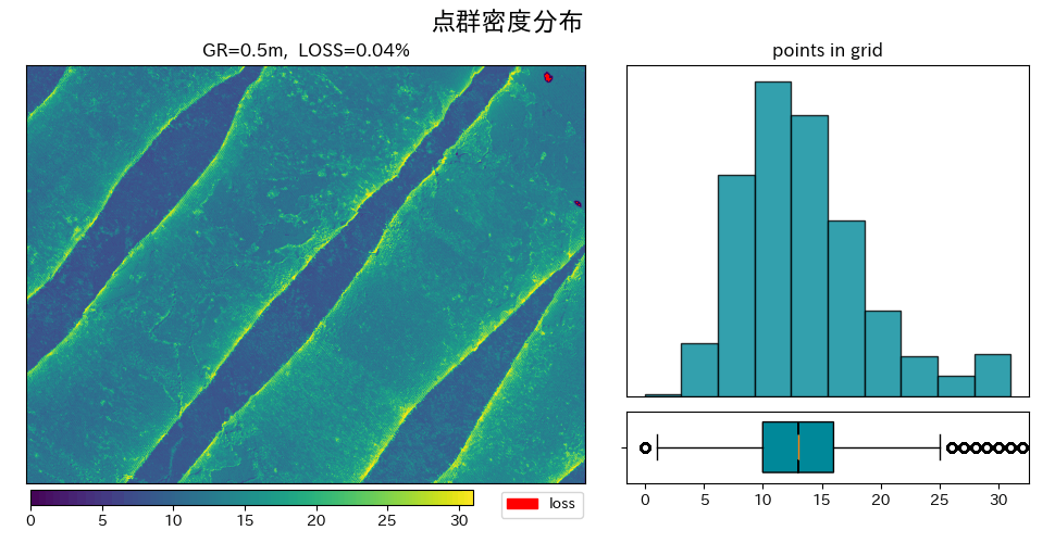
地上分解能0.5mで作成しても特に問題はなさそうです。
3. RGB 画像の作成
3-1. 各パラメーターの設定
実際に画像を作成しますが、Intensity は最大値が 255 なので 8bit ですが、「Red」「Green」「Blue」 の方は最大値が2の16乗の範囲内なので、16bit だと推測できます。別にこのまま出力してもいいですが、使いやすいように 8bit の範囲に変換してしまいましょう。
# 出力ファイルのパスを設定
INTENSITY_PATH = IN_FILE.replace('proj.las', 'INTENSITY.tif')
RED_PATH = IN_FILE.replace('proj.las', 'RED.tif')
GREEN_PATH = IN_FILE.replace('proj.las', 'GREEN.tif')
BLUE_PATH = IN_FILE.replace('proj.las', 'BLUE.tif')
RGB_PATH = IN_FILE.replace('proj.las', 'RGB.tif')

# 地上解像度の設定
RESOLUTION = 0.5

# 16bit の最大値を設定する
_16bit = 2**16 - 1

# 画像として出力する際の設定
write_dict = {
    'type': 'writers.gdal',
    'data_type': 'uint8',
    'resolution': RESOLUTION,
    'output_type': 'mean',
    'nodata': 0,
    'default_srs': IN_SRS,
    'gdaldriver': 'GTiff'
}
3-2. Pipelineの作成と実行
# データの読み込み
readers = readers = pdal.Reader.las(IN_FILE)

# 16bit から 8bit への変換するタスクを構成
fassign = (
    pdal
    .Filter
    .assign(
        value=[
            f'Red = Red / {_16bit} * 255',
            f'Green = Green / {_16bit} * 255',
            f'Blue = Blue / {_16bit} * 255',
        ]
    )
)

paths = [INTENSITY_PATH, RED_PATH, GREEN_PATH, BLUE_PATH]
cols = ['Intensity', 'Red', 'Green', 'Blue']
for path, col in zip(paths, cols):
    # データを書き込むタスクを構成
    writers = (
        pdal
        .Writer(
            filename=path,
            dimension=col,
            **write_dict
        )
    )
    # Pipelineの作成と実行
    pipeline = readers | fassign | writers
    pipeline.execute()
3-3. RGB 配列の作成
rasterio を使用して各色の画像を読み込み read メソッドで配列を取得し、np.dstack で matplotlib で可視化可能な形状にしましょう。
# データの読み込み
intensity_dst = rasterio.open(INTENSITY_PATH)

red_dst = rasterio.open(RED_PATH)

green_dst = rasterio.open(GREEN_PATH)

blue_dst = rasterio.open(BLUE_PATH)

# Raster 形状のデータを作成
rgb_raster = np.array([
    red_dst.read(1),
    green_dst.read(1),
    blue_dst.read(1),
])

# Image 形状のデータに変換
rgb_img = np.dstack(rgb_raster)

print(
f"""
Raster shape: {rgb_raster.shape}
RGB shape   : {rgb_img.shape}
""")
Raster shape: (3, 1501, 2001)
RGB shape   : (1501, 2001, 3)
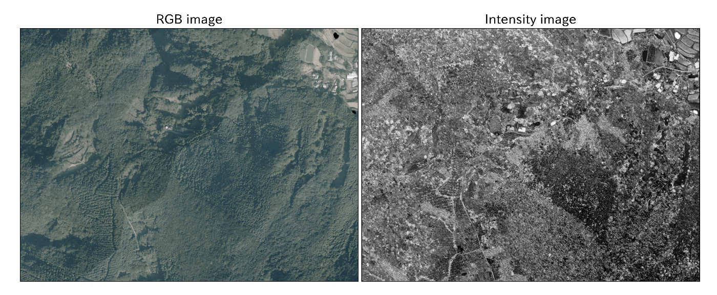
3-4. 画像の確認
それでは上記で作成した RGB と Intensity のデータを matplotlib で表示してみます。
arys = [rgb_img, intensity_dst.read(1)]
titles = ['RGB image', 'Intensity image']

fig, ax = plt.subplots(ncols=2, figsize=(16, 10))
for _ax, ary, title in zip(ax, arys, titles):
    _ax.set_title(title, fontsize=17)
    _ax.imshow(ary, cmap='Grays')
    _ax.axes.xaxis.set_visible(False)
    _ax.axes.yaxis.set_visible(False)

plt.subplots_adjust(wspace=0.01);
4. Rasterの出力
各色の配列を rasterio でまとめて RGB 画像として出力します。画像の範囲などは、事前に読み込んでいたデータからメタデータを取得して使用しますが、'count' の数値は RGB だと 3 枚になるのでそこだけ書き換えます。
metadata = intensity_dst.meta
metadata['count'] = 3
with rasterio.open(RGB_PATH, mode='w', **metadata) as dst:
    for i, _dst in enumerate([red_dst, green_dst, blue_dst]):
        dst.write(_dst.read(1), i + 1)

rgb_dst = rasterio.open(RGB_PATH)
5. Intensity を見てみる
少し Intensity を詳しく見てみましょう。Intensity(反射強度)とは、ポイントを生成しているレーザーパルスが反射される強さを計測し、集計したものです。この数値は「スキャン角度」「粗さ」「含水率」などによって異なります。
調べてみると、反射強度の数値は絶対的な数値ではなく、相対的な数値の様です。その為、同じ場所を計測した場合であっても異なる数値が集計され、正規化された数値を記録している場合がある様です。
rasterio では shapely.Polygon のオブジェクトを使用して画像の切り抜きを行う事が出来るので、幾つかの場所を切り抜き、切り抜いた場所を強調させてみます。
scope_1 = shapely.box(-3250, 38050, -3050, 38200)
scope_2 = shapely.box(-3800, 37650, -3600, 37800)

# 長く読みづらいですが、下記のコードで可視化します。
intensity = intensity_dst.read(1)

fig = plt.figure(figsize=(12, 9))
shape = (6, 6)
# Axis 1
ax1 = plt.subplot2grid(shape, loc=(0, 0), colspan=4, rowspan=4)
ax1.set_title('Intensity image', fontsize=17)
rasterio.plot.show(intensity_dst, cmap='binary_r', ax=ax1)
kwargs = dict(facecolor=(0, 0, 0, 0), linewidth=2, add_points=False)
plot_polygon(scope_1, color='red', **kwargs)
plot_polygon(scope_2, color='blue', **kwargs)

# Axis 2
spans = dict(colspan=2, rowspan=2)
right_kwargs = dict(shapes=[scope_1], crop=True)
ax2 = plt.subplot2grid(shape, loc=(0, 4), **spans)
ax2_img = rasterio.mask.mask(rgb_dst, **right_kwargs)
ax2.imshow(np.dstack(ax2_img[0]))

# Axis 3
ax3 = plt.subplot2grid(shape, loc=(2, 4), **spans)
ax3_img = rasterio.mask.mask(intensity_dst, **right_kwargs)
cb = ax3.imshow(ax3_img[0][0], cmap='binary_r')

# Axis 4
bottom_kwargs = dict(shapes=[scope_2], crop=True)
ax4 = plt.subplot2grid(shape, loc=(4, 0), **spans)
ax4_img = rasterio.mask.mask(rgb_dst, **bottom_kwargs)
ax4.imshow(np.dstack(ax4_img[0]))

# Axis 5
ax5 = plt.subplot2grid(shape, loc=(4, 2), **spans)
ax5_img = rasterio.mask.mask(intensity_dst, **bottom_kwargs)
ax5.imshow(ax5_img[0][0], cmap='binary_r')

# Polygonに合わせてAxisのラインに色を付ける
for _ax, c in zip(fig.axes[1: ], ['red', 'red', 'blue', 'blue']):
    for children in _ax.get_children():
        if isinstance(children, Spine):
            children.set_color(c)

# メモリを消す
for _ax in fig.axes:
    _ax.axes.xaxis.set_visible(False)
    _ax.axes.yaxis.set_visible(False)
    _ax.grid(False)

# Colorbarの表示
cax = inset_axes(
    ax3, width='100%', height='10%',
    bbox_to_anchor=(-0.03, -0.2, 1, 1),
    bbox_transform=ax3.transAxes, loc='lower left'
)
fig.colorbar(cb, cax=cax, orientation="horizontal");
plt.grid(False)
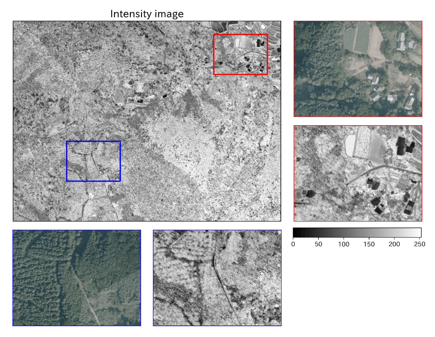
個人的なイメージとしては、屋根や道路の方が反射率が高いかと思っていましたが、上の図を見ると逆の様です。レーザーパルスは近赤外域を使用しているようなので、衛星画像の近赤外域のデータと同じような使い方が出来るのでしょうか。
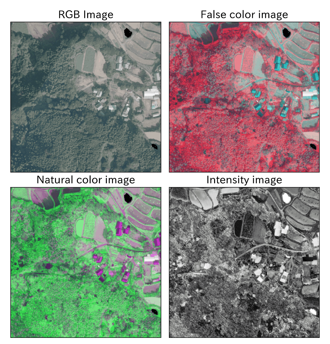
6. バンド合成で遊ぶ
普段よく目にする画像は RGB の画像ですが、各配列の順序を変更したり、別な要素(今回の場合は反射強度)を入力する事で、画像の見た目を変え、注目したいモノを目立たせる事も可能です。
false_ary = np.dstack([
    intensity_dst.read(1),
    red_dst.read(1),
    green_dst.read(1)
])

natural_ary = np.dstack([
    red_dst.read(1),
    intensity_dst.read(1),
    green_dst.read(1)
])

invd_natural_ary = np.dstack([
    (np.array(intensity_dst.read(1).tolist()) - 255) * (-1),
    green_dst.read(1),
    (np.array(intensity_dst.read(1).tolist()) - 255) * (-1)
])

titles = [
    'RGB Image', 'False color image',
    'Natural color image', 'Intensity image'
]
arys = [
    rgb_img, false_ary,
    natural_ary, intensity_dst.read(1),
]


fig = plt.figure(figsize=(9, 9))
for i, (ary, title) in enumerate(zip(arys, titles)):
    ax = fig.add_subplot(2, 2, i + 1)
    ax.set_title(title, fontsize=17)
    ax.imshow(ary[: 600, 1400:], cmap='Grays')
    ax.axes.xaxis.set_visible(False)
    ax.axes.yaxis.set_visible(False)

plt.subplots_adjust(wspace=0, hspace=0.1)
おわりに
今回は点群データから画像を作成する方法と可視化について解説しました。次回は DTM の後処理について考えていきます。
参考
オルソ画像について
PDAL writers.gdal
Processing Autzen Stadium with PDAL and COPC
rasterio document
UAV載型レーザスキャナを用いた公共測量について
LIDAR INTENSITY: WHAT IS IT AND WHAT ARE IT’S APPLICATIONS?
ArcGIS での LIDAR からの強度画像の作成
Discussion