RでGoogle Earth Engineの植生指数時系列データからBFASTによる変化検知を試す
変更履歴・概要
2024/8/13 初版
できるようになること
RからGoogle Earth Engine(GEE)を操作して衛星データをダウンロードし,変化検知に取り組みます。今回は,地表面にいつどのような変化が起きているかについて,衛星データによるタイムラプス動画や植生指数の時系列データのグラフ表示をもとに(直感的に)理解するとともに,統計学的な変化検知手法を用いて(客観的に)示します。
変化検知には,RのBFAST ライブラリを活用します。BFASTは「Breaks for Additive Season and Trend」の略で,オリジナルのBFASTでは時系列データをトレンド,季節性,残差の成分に分解し,成分内での変化を検出することができます。この方法のメリットは,閾値や教師データの設定が不要であり,時系列データのすべてを活用しているという点です。さらに,オリジナルのBFASTに加えて,いくつかの派生したアルゴリズムも紹介します。
https://bfast.r-forge.r-project.org/
https://janverbesselt.github.io/BFASTforAEO/
初期設定
RでGEEを操作する設定は,RでGoogle Earth Engineを操作できるようにするを,光学衛星データを表示する方法は,RでGoogle Earth Engineの光学衛星データを表示するを,それぞれ参考にしてください。
library(rgee)
library(rgeeExtra)
library(tidyverse)
library(tsibble)
library(leaflet)
library(sf)
library(imputeTS)
library(bfast)
ee_Initialize(project = 'プロジェクト名')
eemont <- reticulate::import("eemont")
変化検知を試みた地点
今回は,兵庫県姫路市の夢前スマートIC付近で行います。下記プレスリリースによると,2009(平成21)年9月に工事着手,2015(平成27)年9月に供用開始ですので,(少なくとも)2009年から2015年のいずれかの時点では変化があると考えられます。
https://corp.w-nexco.co.jp/corporate/release/kansai/h27/0805a/
geom_point <- c(134.692408, 34.963211) # https://ja.wikipedia.org/wiki/%E5%A4%A2%E5%89%8D%E3%83%90%E3%82%B9%E3%82%B9%E3%83%88%E3%83%83%E3%83%97
ここでは,次の4箇所の変化検知を行ってみましょう。
point_A <- c(134.692404, 34.962332) # 夢前スマートIC付近
point_B <- c(134.693981, 34.968819) # 太陽光発電設備
point_C <- c(134.701293, 34.969107) # 森林(途中変化あり)
point_D <- c(134.690564, 34.962091) # 森林(途中変化なし)
point_df <- rbind(point_A, point_B, point_C, point_D) %>% as.data.frame()
国土地理院が撮影した最新の空中写真(2020年10~12月撮影)でそれぞれの地点を確認しておきましょう。
leaflet(point_df) %>%
  addTiles("https://cyberjapandata.gsi.go.jp/xyz/seamlessphoto/{z}/{x}/{y}.jpg",
           attribution = "<a href='http://maps.gsi.go.jp/development/ichiran.html' target='_blank'>地理院タイル</a>") %>%
  addPopups(~V1, ~V2, popup = rownames(point_df))

Landsat衛星データの取得
まず,Landsat衛星データの取得を行います。変化検知を行う植生指数としてEVI(Enhanced Vegetation Index)を合わせて取得しておきます。
詳しい方法は,以下のページを参考にしてください。
RでGoogle Earth Engineの光学衛星データをタイムラプス動画として表示する
RによりGoogle Earth Engineの植生指数の地図・時系列データを表示する
EVIについては,以下のページを参考にしてください。
https://en.wikipedia.org/wiki/Enhanced_vegetation_index
## 植生指数
SI <- 'EVI'
## 地点データ:点データから1kmの範囲を設定
ee_geom <- ee$Geometry$Point(geom_point)
ee_geom_buffer <- ee_geom$buffer(1000)
## Landsat5/7のバンド名をLandsat8/9にそろえる関数
rename <- function(image){
  return(image$select(
    c('SR_B1', 'SR_B2', 'SR_B3', 'SR_B4', 'SR_B5', 'SR_B7', SI),
    c('SR_B2', 'SR_B3', 'SR_B4', 'SR_B5', 'SR_B6', 'SR_B7', SI)
  ))
}
## 各衛星データの利用期間
yearStart <- 1995 # filter year included in mosaics.
yearEnd <- 2023 # filter year included in mosaics.
yearInterval <- 1 # if 1 then mosaic every year, if 10 then every 10 years.
years <- seq(yearStart, yearEnd, yearInterval)
monthStart <- 1 # filter months included in mosaics.
monthEnd <- 12 # filter months included in mosaics.
cloudcover <- 50
## 各衛星データの作成
# Landsat5
# https://developers.google.com/earth-engine/datasets/catalog/LANDSAT_LT05_C02_T1_L2
L5_SR <- ee$ImageCollection("LANDSAT/LT05/C02/T1_L2")$
  filterBounds(ee_geom_buffer)$
  filter(ee$Filter$lt('CLOUD_COVER', cloudcover))$
  preprocess()$
  spectralIndices(SI)$
  map(rename)
# Landsat7
# https://developers.google.com/earth-engine/datasets/catalog/LANDSAT_LE07_C02_T1_L2
L7_SR <- ee$ImageCollection("LANDSAT/LE07/C02/T1_L2")$
  filterBounds(ee_geom_buffer)$
  filter(ee$Filter$lt('CLOUD_COVER', cloudcover))$
  preprocess()$
  spectralIndices(SI)$
  map(rename)
# Landsat8
# https://developers.google.com/earth-engine/datasets/catalog/LANDSAT_LC08_C02_T1_L2
L8_SR <- ee$ImageCollection("LANDSAT/LC08/C02/T1_L2")$
  filterBounds(ee_geom_buffer)$
  filter(ee$Filter$lt('CLOUD_COVER', cloudcover))$
  preprocess()$
  spectralIndices(SI)$
  select(c('SR_B2', 'SR_B3', 'SR_B4', 'SR_B5', 'SR_B6', 'SR_B7', SI))
# Landsat9
# https://developers.google.com/earth-engine/datasets/catalog/LANDSAT_LC09_C02_T1_L2
L9_SR <- ee$ImageCollection("LANDSAT/LC09/C02/T1_L2")$
  filterBounds(ee_geom)$
  filter(ee$Filter$lt('CLOUD_COVER', cloudcover))$
  preprocess()$
  spectralIndices(SI)$
  select(c('SR_B2', 'SR_B3', 'SR_B4', 'SR_B5', 'SR_B6', 'SR_B7', SI))
## 各衛星データのマージ
Landsat_SR <- L5_SR$merge(L7_SR)$merge(L8_SR)$merge(L9_SR)$
  filter(ee$Filter$calendarRange(yearStart, yearEnd, "year"))$
  filter(ee$Filter$calendarRange(monthStart, monthEnd, "month"))
タイムラプス動画による確認
タイムラプス動画にして確認してみましょう。
ee_years <- ee$List(years)
createYearlyImage <- function(beginningYear){
  startDate <- ee$Date$fromYMD(beginningYear, 1, 1)
  endDate <- startDate$advance(1, 'year')
  yearFiltered <- Landsat_SR$filter(ee$Filter$date(startDate, endDate))
  total <- yearFiltered$median()$set('system:time_start', startDate$millis())
  return(total)
}
yearlyImages <- ee_years$map(ee_utils_pyfunc(createYearlyImage))
yearlyCollection <- ee$ImageCollection$fromImages(yearlyImages)

imageRGB <- yearlyCollection$map(function(img){
  return(img$visualize(bands=c("SR_B4", "SR_B3", "SR_B2"), min=0, max=0.3))
})

gifParams <- list(
  region = ee_geom_buffer,
  dimensions = 480,
  crs=Landsat_SR$first()$projection()$crs()$getInfo(),
  framesPerSecond = 0.75
)
animation <- ee_utils_gif_creator(imageRGB, gifParams, mode="wb")
get_dates <- ee_get_date_ic(yearlyCollection)
animation_wtxt <- animation %>%
  ee_utils_gif_annotate(format(get_dates$time_start, "%Y"), size=15, location="+20+20", boxcolor = "#FFFFFF") %>%
  ee_utils_gif_annotate("Landsat image courtesy of the U.S. Geological Survey", size=9, location="+240+450", boxcolor = "#FFFFFF")
ee_utils_gif_save(animation_wtxt, path = paste0(zenn_dir, fig_path, "animation-landsat_yearly.gif"))
タイムラプス動画
knitr::include_graphics("images/carook-zenn-r-rgee06/animation-landsat_yearly.gif", error=F)
変化検知に向けた前処理
タイムラプス動画からは,point_Aは2012~2013年頃,point_Bは2018~2019年頃,point_Cは2011~2012年頃に変化し,point_C付近のみ植生が回復しているとみられます。point_Dは森林のまま変化がないとみられる地点です。それでは,データをRに取り込んで変化検知を行ってみましょう。
変化検知用のデータ取得
eemontのgetTimeSeriesByRegions()でデータを抽出し,ee_as_sf()でRのsfオブジェクトに変換(ダウンロード)しています。
Landsat_SR_SI_toR <- Landsat_SR %>%
  ee$ImageCollection$getTimeSeriesByRegions(
    reducer = ee$Reducer$mean(),
    collection= ee$FeatureCollection(list(
      ee$Feature(ee$Geometry$Point(point_A), list(name="point_A")),
      ee$Feature(ee$Geometry$Point(point_B), list(name="point_B")),
      ee$Feature(ee$Geometry$Point(point_C), list(name="point_C")),
      ee$Feature(ee$Geometry$Point(point_D), list(name="point_D"))
      )),
    bands = SI,
    scale = 30) %>%
  ee_as_sf() %>%
  mutate_at(vars(all_of(SI)), na_if, -9999) %>% # -9999はNAに置換
  sf::st_drop_geometry() %>% # geometry情報は不要なので削除
  select(SI = 1, dplyr::everything())%>% # 値の列名をSIとする
  mutate(SI=case_when(SI < 0 ~ as.numeric(NA), # SI < 0 であればNAに置換
                      SI > 1 ~ as.numeric(NA), # SI > 1 であればNAに置換
                      TRUE ~ SI)) %>%
  drop_na(everything()) # NAを除去
グラフとして表示してみると,次のとおりになります。
ggplot(Landsat_SR_SI_toR, aes(x=date, y=SI, colour=name)) +
  geom_point(size=1) +
  geom_smooth(linewidth=1.5, se = FALSE, span = 0.1) +
  ylim(c(0,1)) + ylab(SI) +
  scale_x_datetime(date_breaks="2 year", date_labels="%y/%m") +
  theme(legend.position="bottom")

ts形式への変換
BFASTではデータをts形式に変換しておく必要があります。ts形式への変換の前段階として,data.frame形式からtsibble形式に変換し,日単位では欠損値が多すぎるので,月ごとの平均値に集計しておきます。tsibble形式はtibble(tbl_df)形式を時系列データを扱えるように拡張した形式と理解しておけば良さそうです。詳しくは以下のページをご覧ください。
https://tsibble.tidyverts.org/
SI_yearmonth <- Landsat_SR_SI_toR %>%
  as_tsibble(key=name, regular=FALSE) %>%
  group_by(name) %>%
  index_by(Year_Month = ~ yearmonth(.)) %>%
  summarise(
    Mean_SI = mean(SI)
  )
## Using `date` as index variable.
class(SI_yearmonth)
## [1] "tbl_ts" "tbl_df" "tbl" "data.frame"
グラフとして表示してみましょう。
ggplot(SI_yearmonth, aes(x=Year_Month, y=Mean_SI, colour=name)) +
  geom_point(size=1) +
  geom_smooth(linewidth=1.5, se = FALSE, span = 0.1) +
  ylim(c(0,1)) + ylab(SI) +
  scale_x_yearmonth(date_breaks="2 year", date_labels="%y/%m") +
  theme(legend.position="bottom")

ts形式とするため,tsibbleライブラリのas.ts()で変換します。
SI_ts <- SI_yearmonth %>% as.ts()
class(SI_ts)
## [1] "mts" "ts" "matrix" "array"
参考:あらかじめts形式に変換しない方法
ts形式に変換せず,bfastライブラリのbfastts関数を利用して以下のようにts形式のデータを変換してもよいのですが,関数のヘルプによると,うるう年の処理に難がありそうなので,今回は用いていません。
bfastts(data=Landsat_SR_SI_toR$SI, dates=as.Date(Landsat_SR_SI_toR$date), type=c("irregular"))
BFASTによる変化検知
オリジナルのBFAST
まずは,オリジナルのBFASTから紹介します。
Verbesselt J, Hyndman R, Newnham G, Culvenor D (2010) Detecting trend and seasonal changes in satellite image time series. Remote Sens Environ 114:106–115. https://doi.org/10.1016/j.rse.2009.08.014
Verbesselt J, Hyndman R, Zeileis A, Culvenor D (2010) Phenological change detection while accounting for abrupt and gradual trends in satellite image time series. Remote Sens Environ 114:2970–2980. https://doi.org/10.1016/j.rse.2010.08.003
欠損値を扱えないので,imputeTSライブラリを利用してスプライン補間した上で,解析を行います。
SI_ts_spline <- SI_ts %>%
  imputeTS::na_interpolation(option = "spline")
bfast中のhはトレンド成分についての変化検知の最小間隔で,標本サイズに対する割合で与えます。ここでは5年(5*12=60月)としました。
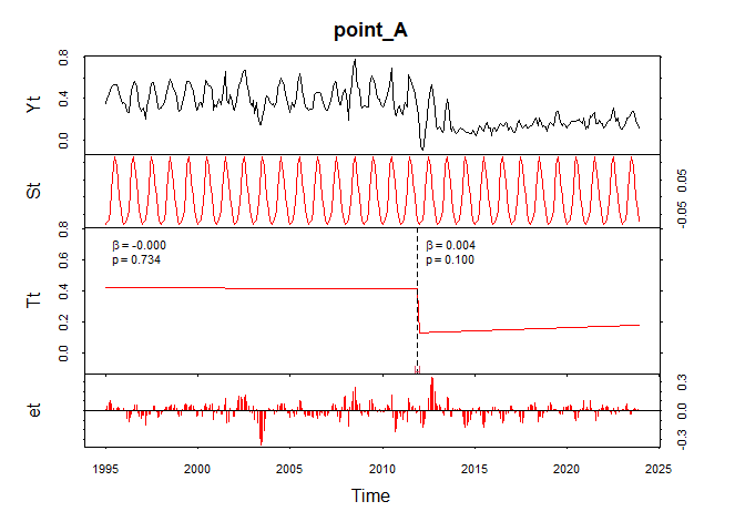
図の一番上のYtが元の時系列データ,Stが季節性成分,Ttがトレンド成分,etが残差成分をそれぞれ示しています。検知した変化は赤い点線で示されており,図の下側には変化した時点の信頼区間があわせて示されています。各地点で,トレンド成分にいくつかの変化が検知されています。
なおver1.6.0からdecomp="stlplus"とすることで欠損値の補間なしに各成分への分解を行うことも可能です(が,変化検知が示されていない?)。
for(i in 1:nrow(point_df)){
  bp <- bfast(SI_ts_spline[,i], h= 60/length(SI_ts_spline[,i]), season="harmonic", decomp="stl")
  plot(bp, ANOVA=T, main=rownames(point_df)[i])
}


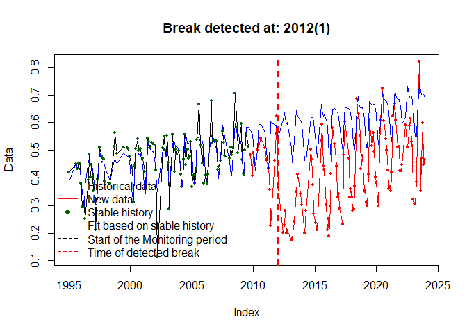
BFAST Monitor
BFAST Monitorは時系列データのなかで直近の変化を検知するためのアルゴリズムです。過去の安定的な時系列データに基づいて作成されたモデルによって,新しく取得したデータ(モニタリング期間)内の変化を検知することが可能になります。ただし,変化しているかどうかが主な注目点で,その時期については精度が多少劣るようです。詳しくは以下の文献で確認してください。
Verbesselt J, Zeileis A, Herold M (2012) Near real-time disturbance detection using satellite image time series. Remote Sens Environ 123:98–108. https://doi.org/10.1016/j.rse.2012.02.022
bfastmonitorのstartによってモニタリング期間の開始時期を設定します。黒がモデル作成期間のデータ,赤がモニタリング期間のデータ,青はモデルによる推定値,黒い点線がモニタリング期間の開始時期,赤い点線が変化検知された時期をそれぞれれ示しています。
for(i in 1:nrow(point_df)){
  par(mfrow=c(1,1))
  bfm <- bfastmonitor(SI_ts[,i], start = c(2009,9))
  plot(bfm)
}


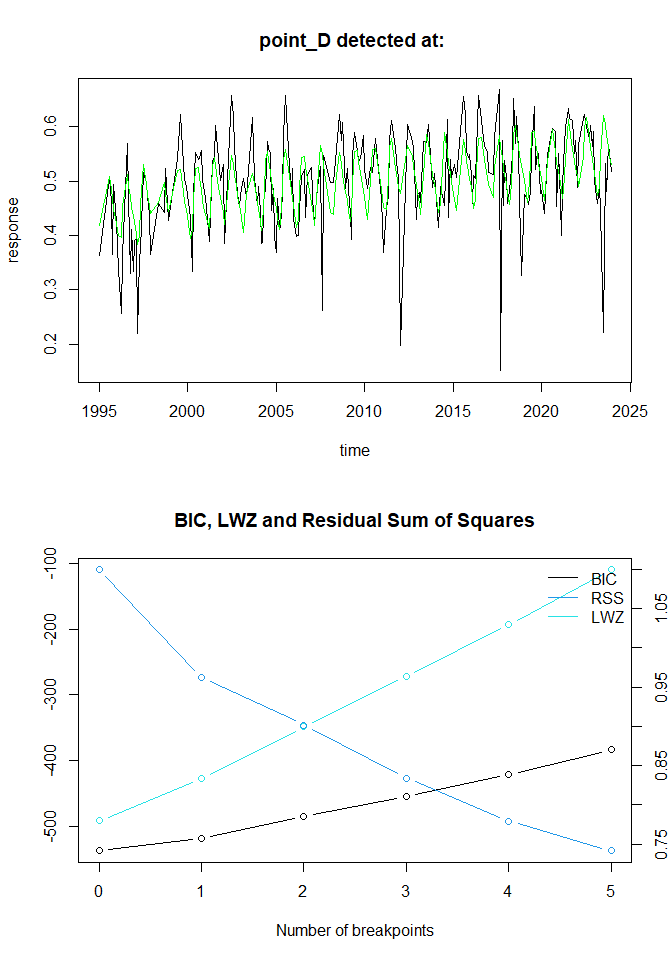
BFAST Lite
最後に,BFASTの軽量版として開発されたBFAST Liteを紹介します。オリジナルのBFASTのようにトレンドと季節性に時系列データを分解することはできませんが,高速で欠損値を扱えるという利点があります。詳しくは,以下の文献で確認してください。
Masiliūnas D, Tsendbazar N-E, Herold M, Verbesselt J (2021) BFAST Lite: A Lightweight Break Detection Method for Time Series Analysis. Remote Sens 13:3308. https://doi.org/10.3390/rs13163308
上のグラフの黒い線が元の時系列データ,緑色の線がモデルによる推定値,青い縦線が変化検知された時期を示しています。タイトルにも最初に検知された時期を示しています。下のグラフは横軸に変化検知した数,縦軸に各情報指数の値をとったものです。RSS(残差平方和)は変化検知数が増えるほど減っていますが,不必要に多い変化検知数を採択することにペナルティーを課すため,LWZ(もしくはBIC)が最小の変化検知数を採択することになります。
bp <- list()
for(i in 1:nrow(point_df)){
  bp[[i]] <- bfastlite(SI_ts[,i])

  if(is.na(bp[[i]]$breakpoints$breakpoints[1])){
    yearmon.bp <- NULL
  } else{
    yearmon.no.na <- tibble(x=as.numeric(time(SI_ts[,i])), y=as.vector(SI_ts[,i])) %>%
      drop_na(everything())
    yearmon.bp <- as.yearmon(yearmon.no.na[bp[[i]]$breakpoints$breakpoints[1],1]) %>%
      format("%Y %b")
  }

  par(mfrow=c(2,1))
  plot(bp[[i]], main=paste(rownames(point_df)[i], "detected at:", yearmon.bp))
  plot(bp[[i]]$breakpoints)
}


magnitude関数によって,検知した変化の特徴をみることができます。ここでは,point_Bのみを表示しています。
magnitude(bp[[2]]$breakpoints)
## $Mag
##         before    after       diff     RMSD       MAD         MD
## [1,] 0.4990562 0.125076 -0.3739802 0.373467 0.3724613 -0.3724613
##
## $m.x
## [1] 186 186
##
## $m.y
##    before     after
## 0.4990562 0.1250760
##
## $Magnitude
##       diff
## -0.3739802
##
## $Time
## [1] 186
##
## attr(,"class")
## [1] "magnitude"
Session info
sessionInfo()
## R version 4.3.3 (2024-02-29 ucrt)
## Platform: x86_64-w64-mingw32/x64 (64-bit)
## Running under: Windows 10 x64 (build 19045)
##
## Matrix products: default
##
##
## locale:
## [1] LC_COLLATE=Japanese_Japan.utf8  LC_CTYPE=Japanese_Japan.utf8    LC_MONETARY=Japanese_Japan.utf8
## [4] LC_NUMERIC=C                    LC_TIME=Japanese_Japan.utf8
##
## time zone: Etc/GMT-9
## tzcode source: internal
##
## attached base packages:
## [1] stats     graphics  grDevices utils     datasets  methods   base
##
## other attached packages:
##  [1] bfast_1.6.1                 strucchangeRcpp_1.5-3-1.0.4 sandwich_3.1-0              zoo_1.8-12
##  [5] sf_1.0-16                   leaflet_2.2.2               tsibble_1.1.5               lubridate_1.9.3
##  [9] forcats_1.0.0               stringr_1.5.1               dplyr_1.1.4                 purrr_1.0.2
## [13] readr_2.1.5                 tidyr_1.3.1                 tibble_3.2.1                ggplot2_3.5.1
## [17] tidyverse_2.0.0             rgeeExtra_0.0.1             rgee_1.1.7                  here_1.0.1
## [21] fs_1.6.4                    rmarkdown_2.26
##
## loaded via a namespace (and not attached):
##   [1] rstudioapi_0.16.0     jsonlite_1.8.8        magrittr_2.0.3        magick_2.8.3          farver_2.1.1
##   [6] vctrs_0.6.5           memoise_2.0.1         base64enc_0.1-3       terra_1.7-71          webshot_0.5.5
##  [11] htmltools_0.5.8.1     usethis_2.2.3         curl_5.2.1            raster_3.6-26         TTR_0.24.4
##  [16] KernSmooth_2.23-22    htmlwidgets_1.6.4     plyr_1.8.9            cachem_1.0.8          mime_0.12
##  [21] lifecycle_1.0.4       pkgconfig_2.0.3       webshot2_0.1.1        Matrix_1.6-5          R6_2.5.1
##  [26] fastmap_1.1.1         rbibutils_2.2.16      shiny_1.8.1.1         digest_0.6.34         colorspace_2.1-0
##  [31] RODBC_1.3-23          ps_1.7.6              rprojroot_2.0.4       leafem_0.2.3          pkgload_1.3.4
##  [36] crosstalk_1.2.1       geojson_0.3.5         labeling_0.4.3        imputeTS_3.3          timechange_0.3.0
##  [41] fansi_1.0.6           mgcv_1.9-1            httr_1.4.7            compiler_4.3.3        microbenchmark_1.4.10
##  [46] proxy_0.4-27          remotes_2.5.0         bit64_4.0.5           withr_3.0.0           tseries_0.10-56
##  [51] DBI_1.2.2             highr_0.10            pkgbuild_1.4.4        protolite_2.3.0       stinepack_1.5
##  [56] sessioninfo_1.2.2     classInt_0.4-10       chromote_0.2.0        tools_4.3.3           units_0.8-5
##  [61] lmtest_0.9-40         odbc_1.4.2            quantmod_0.4.26       httpuv_1.6.15         nnet_7.3-19
##  [66] glue_1.7.0            quadprog_1.5-8        nlme_3.1-164          promises_1.3.0        gridtext_0.1.5
##  [71] grid_4.3.3            geojsonio_0.11.3      generics_0.1.3        gtable_0.3.5          tzdb_0.4.0
##  [76] class_7.3-22          websocket_1.4.1       hms_1.1.3             sp_2.1-4              xml2_1.3.6
##  [81] utf8_1.2.4            pillar_1.9.0          later_1.3.2           splines_4.3.3         ggtext_0.1.2
##  [86] lattice_0.22-5        bit_4.0.5             tidyselect_1.2.1      miniUI_0.1.1.1        knitr_1.46
##  [91] V8_4.4.2              urca_1.3-4            crul_1.4.2            forecast_8.23.0       xfun_0.43
##  [96] devtools_2.4.5        timeDate_4032.109     DT_0.33               stringi_1.8.3         geojsonsf_2.0.3
## [101] lazyeval_0.2.2        ggmap_4.0.0           yaml_2.3.8            httpcode_0.3.0        evaluate_0.23
## [106] codetools_0.2-19      cli_3.6.1             Rdpack_2.6            xtable_1.8-4          reticulate_1.35.0
## [111] jquerylib_0.1.4       munsell_0.5.1         processx_3.8.4        jqr_1.3.3             Rcpp_1.0.12
## [116] anytime_0.3.9         png_0.1-8             parallel_4.3.3        ellipsis_0.3.2        fracdiff_1.5-3
## [121] blob_1.2.4            jpeg_0.1-10           profvis_0.3.8         urlchecker_1.0.1      bitops_1.0-7
## [126] scales_1.3.0          xts_0.14.0            e1071_1.7-14          crayon_1.5.2          rlang_1.1.3
Discussion