RでGoogle Earth Engineの光学衛星データをダウンロードする


変更履歴・概要
2024/3/28 初版
できるようになること
Google Earth Engine(GEE)からデータをダウンロードし,R上で処理できるようにします。 ここでは参考として,rayshaderライブラリを利用した3D画像を作成してみます。
初期設定
RでGEEを操作する設定は,RでGoogle Earth Engineを操作できるようにするを,光学衛星データを表示する方法は,RでGoogle Earth Engineの光学衛星データを表示するを,それぞれ参考にしてください。
GEEから直接ローカルにダウンロードすることはできません。GoogleDriveもしくはGoogle Cloud Stroageのいずれかに保存してから,ローカルにデータを移すことになります。以下のページに,GEEからの衛星画像の出力に関する説明があるので一読することをおすすめします。
https://developers.google.com/earth-engine/guides/exporting_images
ここではGoogleDriveへの保存を行うため,ee_Initialize()でdrive=Tと設定します。
library(rgee)
library(rgeeExtra)
library(terra)
library(rayshader)
library(tmap)
library(leaflet)
library(magick)
ee_Initialize(project = 'プロジェクト名', drive = T)
(参考)rmarkdownで3D画像を保存する
ここで紹介するrayshaderライブラリのplot_3D()ではrglライブラリを利用することで3D画像を作成します。通常の設定では,別ウィンドウが開いて3D画像が表示されますが,rmarkdownライブラリを利用した原稿出力には不要なので,rglライブラリを読み込む前に以下により,画面出力をさせないようにしています。
あわせてrglオブジェクトの出力を可能にするためsetupKnitr()の設定を行っています(ここでは静止画像の出力なのでなくてもよさそうですが)。
options(rgl.useNULL = TRUE)
library(rgl)
setupKnitr(autoprint = TRUE)
https://cran.r-project.org/web/packages/rgl/vignettes/rgl.html
(参考)rgeeでローカルにデータを出力できない場合
私の環境では,当初ee_as_**でGoogleDriveにはデータが出力されても,drive_auth()に関するエラーによりローカルにデータが来ない現象が起きました。以下のページの記載をもとに,一旦認証情報を削除してから,Rを再起動して再度認証を行うことで出力が可能になりました。エラーが出た場合の参考になればと思います。(多分,これ以外にもいろいろエラーが起きる要因がありそう・・・)
https://github.com/r-spatial/rgee/issues/271
ee_clean_user_credentials(user="ndef")
衛星データ(Image)のダウンロード
ダウンロードするためのデータをGEE上に作成します。
出力範囲を決めます。
geom_rect <- list(c(135.12, 34.82), c(135.12, 34.62),
                  c(135.42, 34.62), c(135.42, 34.82), c(135.12, 34.82))
ee_geom_rect <-  ee$Geometry$Polygon(geom_rect)
ee_geom_rect_centroid <- ee_geom_rect$centroid('maxError' = 1)
centroid <- ee_geom_rect_centroid$coordinates()$getInfo()
Landsat-8のデータを利用します。ここでは,データを表示用に変換しています。コードの説明は,RでGoogle Earth Engineの光学衛星データを表示するで確認してください。
L8_SR <- ee$ImageCollection("LANDSAT/LC08/C02/T1_L2")$
  filterDate("2023-01-01", "2024-01-01")$
  filterBounds(ee_geom_rect)$
  filter(ee$Filter$lt('CLOUD_COVER', 50))$
  preprocess()
L8_SR_RGB <- L8_SR$median()$visualize(bands=c("SR_B4", "SR_B3", "SR_B2"), min=0, max=0.3)
GEE上で,表示させてみます。
Map$setCenter(lon = centroid[1], lat = centroid[2], zoom = 10)
m <- Map$addLayer(L8_SR_RGB) +
  Map$addLayer(ee_geom_rect, list(color = "FF0000"), "geodesic polygon")
m %>%
  leaflet::addTiles(urlTemplate = "", attribution = '| Landsat-8 image courtesy of the U.S. Geological Survey')

ローカルに(直接)保存する
rgeeではImageからraster,stars,SpatRasterの形式で出力する関数が用意されています。後で紹介するrayshaderライブラリで利用できるのはrasterとSpatRasterで,rasterは今後廃止される見通しのため,SpatRasterで出力します。
imageで出力したい衛星データ,regionで出力する範囲を指定します。dsnに出力ファイル名を入れておくと,ファイルがgetwd()で得られるフォルダに保存されます(空欄の場合でも,テンポラリファイルが出力されてR上でデータを利用できますが,複数のデータは同時に利用できません)。crsで座標系,crsTransformでピクセルグリッドのパラメーターを設定します。scale(メートル単位)を指定することでcrsTransformパラメータは自動計算されますが,原点が特定されないため,他のデータとの重ね合わせ時にずれる要因となります(https://developers.google.com/earth-engine/guides/exporting_images)。
SR_proj <- L8_SR$first()$select('SR_B2')$projection()$getInfo()
SR_RGB <- ee_as_rast(image=L8_SR_RGB,
                     region=ee_geom_rect,
                     dsn='rgee05_out/SR_RGB.tif',
                     crs=SR_proj$crs,
                     crsTransform=SR_proj$transform)
## Registered S3 method overwritten by 'geojsonsf':
##   method        from
##   print.geojson geojson

## - region parameters
##  sfg      : POLYGON ((135.12 34.62, 135 .... 135.12 34.82, 135.12 34.62))
##  CRS      : GEOGCRS["WGS 84",
##     DATUM["World Geodetic System 1984",
##         ELLIPSOID["WGS 84",6378137,298.257223563, .....
##  geodesic : TRUE
##  evenOdd  : TRUE
##
## - download parameters (Google Drive)
##  Image ID    : SR_RGB
##  Google user : ndef
##  Folder name : rgee_backup
##  Date        : 2024_03_28_22_23_34
## Polling for task <id: X5E5CW4CANGY33WARPKLQQID, time: 0s>.
## Polling for task <id: X5E5CW4CANGY33WARPKLQQID, time: 5s>.
## Polling for task <id: X5E5CW4CANGY33WARPKLQQID, time: 10s>.
## Polling for task <id: X5E5CW4CANGY33WARPKLQQID, time: 15s>.
## State: COMPLETED
## Moving image from Google Drive to Local ... Please wait

## Auto-refreshing stale OAuth token.
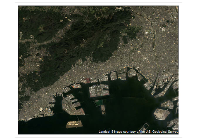
R上で表示してみましょう。表示だけであれば,terra::plotRGB(SR_RGB)でよいのですが,ここではcredit情報を表示させるためtmapライブラリを利用しています。
SR_RGB
## class       : SpatRaster
## dimensions  : 743, 919, 3  (nrow, ncol, nlyr)
## resolution  : 30, 30  (x, y)
## extent      : 510945, 538515, 3830895, 3853185  (xmin, xmax, ymin, ymax)
## coord. ref. : WGS 84 / UTM zone 53N (EPSG:32653)
## source      : SR_RGB.tif
## colors RGB  : 1, 2, 3
## names       : vis-red, vis-green, vis-blue
tm_shape(SR_RGB) + tm_rgb(r=1, g=2, b=3) +
  tm_credits("Landsat-8 image courtesy of the U.S. Geological Survey",
             col="#FFFFFF", position=c("right", "bottom"))
(参考)(表示用でない)元データのダウンロード
(表示用でない)元のデータをダウンロードすることもできます。
L8_local <- ee_as_rast(image=L8_SR$median(),
                       region=ee_geom_rect,
                       dsn='L8_local.tif',
                       crs=SR_proj$crs,
                       crsTransform=SR_proj$transform,
                       lazy=T)
lazy=Tとすることで,タスクがモニタされず,複数のタスクを同時に実行できます。この場合のデータの取り出しは以下により行います。
L8_result <- L8_local %>% ee_utils_future_value()
terra::plotRGB(L8_result, r=4, g=3, b=2, stretch='lin')
GoogleDriveに保存後ローカルに出力
GoogleDriveに保存,GoogleDriveからローカルへのダウンロードと2段階に分けることもできます。まず,GoogleDriveへの保存は以下により行います。
task_img <- ee_image_to_drive(
  image = L8_SR_RGB,
  folder = "rgee_backup",
  fileFormat = "GEO_TIFF",
  region = ee_geom_rect,
  crs=SR_proj$crs,
  crsTransform=SR_proj$transform,
  fileNamePrefix = "my_image_demo"
)
task_img$start()
ee_monitoring(task_img)
GoogleDriveからローカルへのダウンロードを行います。
img <- ee_drive_to_local(task = task_img, dsn='SR_RGB.tif')
得られるオブジェクトはローカルファイル名の文字列です。読み込みの例は以下のとおりです(図は省略)。
class(img)
img_rast <- rast(img)
terra::plotRGB(img_rast)
なお,GoogleDriveのフォルダは以下で削除できます。
ee_clean_container(name = "rgee_backup", type = "drive", quiet = FALSE)
光学衛星データの3D表示
光学衛星データとDEMデータを用いて,rayshaderライブラリを利用し3D表示を行ってみます。
http://www.malikarrahiem.com/making-3d-maps-of-sentinel-2-imagery-with-rayshader/
DEMデータの3D表示
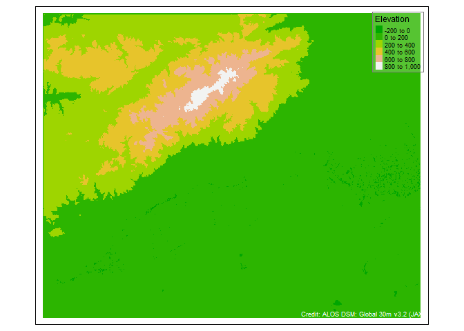
DEMデータはJAXAが整備しているALOS全球数値地表モデル (DSM) “ALOS World 3D - 30m (AW3D30)”を利用します。このデータセットはImageCollectionなので,データ表示にはmosaic()によりImageにしておきます。
AW3D30 <- ee$ImageCollection('JAXA/ALOS/AW3D30/V3_2')
AW3D30.DSM <- AW3D30$select('DSM')$mosaic()
rgeeライブラリを利用してSpatRasterで出力します。
AW3D30.DSM.local <- ee_as_rast(image=AW3D30.DSM,
                               region=ee_geom_rect,
                               crs=SR_proj$crs,
                               crsTransform=SR_proj$transform)
## - region parameters
##  sfg      : POLYGON ((135.12 34.62, 135 .... 135.12 34.82, 135.12 34.62))
##  CRS      : GEOGCRS["WGS 84",
##     DATUM["World Geodetic System 1984",
##         ELLIPSOID["WGS 84",6378137,298.257223563, .....
##  geodesic : TRUE
##  evenOdd  : TRUE
##
## - download parameters (Google Drive)
##  Image ID    : noid_image
##  Google user : ndef
##  Folder name : rgee_backup
##  Date        : 2024_03_28_22_24_21
## Polling for task <id: RFVOYEFTSYKRIQTANXYDFIAG, time: 0s>.
## Polling for task <id: RFVOYEFTSYKRIQTANXYDFIAG, time: 5s>.
## Polling for task <id: RFVOYEFTSYKRIQTANXYDFIAG, time: 10s>.
## State: COMPLETED
## Moving image from Google Drive to Local ... Please wait
R上で表示してみましょう。
AW3D30.DSM.local
## class       : SpatRaster
## dimensions  : 743, 919, 1  (nrow, ncol, nlyr)
## resolution  : 30, 30  (x, y)
## extent      : 510945, 538515, 3830895, 3853185  (xmin, xmax, ymin, ymax)
## coord. ref. : WGS 84 / UTM zone 53N (EPSG:32653)
## source      : noid_image.tif
## name        : DSM
tm_shape(AW3D30.DSM.local) + tm_raster(palette = terrain.colors(10), title='Elevation') +
  tm_layout(scale = .8,
            legend.position = c("right","top"),
            legend.bg.color = "white", legend.bg.alpha = .2,
            legend.frame = "gray50") +
  tm_credits("Credit: ALOS DSM: Global 30m v3.2 (JAXA)",
             col="#FFFFFF", position=c("right", "bottom"))
rayshaderライブラリで利用できる行列データに変換します。
elmat = raster_to_matrix(AW3D30.DSM.local)
## [1] "Dimensions of matrix are: 743x919"
rayshaderライブラリで,2次元画像を表示させてみます。今回は説明を省略しますが,地形表現を色々変えることもできます。
elmat %>%
  sphere_shade(texture = "imhof1") %>%
  plot_map(title_text = "ALOS DSM: Global 30m v3.2 (JAXA)",
           title_size = 20, title_position = "southwest",
           title_bar_color = "white", title_color = "black", title_bar_alpha = )

3Dで表示させてみます。
elmat %>%
  sphere_shade(texture = "imhof1") %>%
  add_water(detect_water(elmat), color = "imhof1") %>%
  add_shadow(ray_shade(elmat, zscale = 3), 0.5) %>%
  add_shadow(ambient_shade(elmat), 0) %>%
  plot_3d(elmat, zscale = 10, fov = 0, theta = 135, zoom = 0.75, phi = 45, windowsize = c(1000, 800))
Sys.sleep(0.2)
render_snapshot(title_text = "ALOS DSM: Global 30m v3.2 (JAXA)",
                title_size = 20, title_position = "southwest",
                title_bar_color = "white", title_color = "black", title_bar_alpha = 1)

光学衛星データの3D表示
光学衛星データは,Landsat8データから上で作成したSR_RGBを用います。まずは,3D画像として重ね合わせるためのデータを作成します。
names(SR_RGB) = c("r","g","b")
mask_r = rayshader::raster_to_matrix(SR_RGB$r)
## [1] "Dimensions of matrix are: 743x919"
mask_g = rayshader::raster_to_matrix(SR_RGB$g)
## [1] "Dimensions of matrix are: 743x919"
mask_b = rayshader::raster_to_matrix(SR_RGB$b)
## [1] "Dimensions of matrix are: 743x919"
mask_array = array(0,dim=c(nrow(mask_r),ncol(mask_r),3))
mask_array[,,1] = mask_r/255 #Red layer
mask_array[,,2] = mask_g/255 #Blue layer
mask_array[,,3] = mask_b/255 #Green layer
mask_array = aperm(mask_array, c(2,1,3))
3D画像は以下により作成します。
plot_3d(mask_array, elmat,
        windowsize = c(1100,900),
        zscale = 10, fov = 0, theta = 300, zoom = 0.75, phi = 15)
render_snapshot(title_text = "Imagery: Landsat-8 | ALOS DSM: Global 30m v3.2 (JAXA)",
                title_size = 20, title_position = "southwest",
                title_bar_color = "white", title_color = "black", title_bar_alpha = 1)

衛星データ(ImageCollection)の出力と活用
ImageCollectionでも出力可能です。以下を参考に,出力した画像を元に3Dのライムラプス動画を作成してみます。
https://bevingtona.github.io/20210504_rgee_rayshade_gifski.html
データの取得と前処理を行います。詳しくは,RでGoogle Earth Engineの光学衛星データをタイムラプス動画として表示するを参考にしてください。
geom_rect <- list(c(135.12, 34.82), c(135.12, 34.62),
                  c(135.42, 34.62), c(135.42, 34.82), c(135.12, 34.82))
ee_geom_rect <-  ee$Geometry$Polygon(geom_rect)
ee_geom_rect_centroid <- ee_geom_rect$centroid('maxError' = 1)
centroid <- ee_geom_rect_centroid$coordinates()$getInfo()
## 各衛星データの利用期間
yearStart <- 1985 # filter year included in mosaics.
yearEnd <- 2023 # filter year included in mosaics.
yearInterval <- 5 # if 1 then mosaic every year, if 10 then every 10 years.
years <- seq(yearStart, yearEnd, yearInterval)
monthStart <- 1 # filter months included in mosaics.
monthEnd <- 12 # filter months included in mosaics.
cloudcover <- 50
## 各衛星データの作成
rename <- function(image){
  return(image$select(
    c('SR_B1', 'SR_B2', 'SR_B3', 'SR_B4', 'SR_B5', 'SR_B7'),
    c('SR_B2', 'SR_B3', 'SR_B4', 'SR_B5', 'SR_B6', 'SR_B7')
  ))
}
# Landsat5
# https://developers.google.com/earth-engine/datasets/catalog/LANDSAT_LT05_C02_T1_L2
L5_SR <- ee$ImageCollection("LANDSAT/LT05/C02/T1_L2")$
  filterBounds(ee_geom_rect)$
  filter(ee$Filter$lt('CLOUD_COVER', cloudcover))$
  preprocess()$
  map(rename)
# Landsat7
# https://developers.google.com/earth-engine/datasets/catalog/LANDSAT_LE07_C02_T1_L2
L7_SR <- ee$ImageCollection("LANDSAT/LE07/C02/T1_L2")$
  filterBounds(ee_geom_rect)$
  filter(ee$Filter$lt('CLOUD_COVER', cloudcover))$
  preprocess()$
  map(rename)
# Landsat8
# https://developers.google.com/earth-engine/datasets/catalog/LANDSAT_LC08_C02_T1_L2
L8_SR <- ee$ImageCollection("LANDSAT/LC08/C02/T1_L2")$
  filterBounds(ee_geom_rect)$
  filter(ee$Filter$lt('CLOUD_COVER', cloudcover))$
  preprocess()$
  select(c('SR_B2', 'SR_B3', 'SR_B4', 'SR_B5', 'SR_B6', 'SR_B7'))
## 各衛星データのマージ
Landsat_SR <- L5_SR$merge(L7_SR)$merge(L8_SR)$
  filter(ee$Filter$calendarRange(yearStart, yearEnd, "year"))$
  filter(ee$Filter$calendarRange(monthStart, monthEnd, "month"))
SR_proj <- Landsat_SR$first()$select('SR_B2')$projection()$getInfo()
## 年ごとの集計
ee_years <- ee$List(years)
createYearlyImage <- function(beginningYear){
  startDate <- ee$Date$fromYMD(beginningYear, 1, 1)
  endDate <- startDate$advance(1, 'year')
  yearFiltered <- Landsat_SR$filter(ee$Filter$date(startDate, endDate))
  total <- yearFiltered$median()$set('system:time_start', startDate$millis())
  return(total)
}
yearlyImages <- ee_years$map(ee_utils_pyfunc(createYearlyImage))
yearlyCollection <- ee$ImageCollection$fromImages(yearlyImages)
## 表示の設定
imageRGB <- yearlyCollection$map(function(img){
  return(img$visualize(bands=c("SR_B4", "SR_B3", "SR_B2"), min=0, max=0.3))
})
作成したデータと動画範囲の確認
Map$setCenter(lon = centroid[1], lat = centroid[2], zoom = 11)
m <- Map$addLayer(imageRGB$first())+
  Map$addLayer(ee_geom_rect, list(color = "FF0000"), "geodesic polygon")
m %>%
  addTiles(urlTemplate = "", attribution = '| Landsat image courtesy of the U.S. Geological Survey')

ImageCollectionの出力には,rgeeライブラリのee_imagecollection_to_local()を利用できます。ただし,crsの設定はできないようです。
ic_drive_files <- ee_imagecollection_to_local(
  ic = imageRGB,
  region = ee_geom_rect,
  dsn = "out/yearly_",
  scale=30
)
そこで,上で紹介したコードを活かして,各年の衛星画像から3D画像を作成させることにします。
lapply(years, function(year) {
  yr <- yearlyCollection$filter(ee$Filter$calendarRange(year, year, "year"))$first()
  yr_RGB <- yr$visualize(bands=c("SR_B4", "SR_B3", "SR_B2"), min=0, max=0.3)
  SR_RGB <- ee_as_rast(image=yr_RGB,
                       region=ee_geom_rect,
                       dsn=paste0('rgee05_out/SR_RGB_', year,'.tif'),
                       crs=SR_proj$crs,
                       crsTransform=SR_proj$transform)
  names(SR_RGB) = c("r","g","b")
  mask_r = rayshader::raster_to_matrix(SR_RGB$r)
  mask_g = rayshader::raster_to_matrix(SR_RGB$g)
  mask_b = rayshader::raster_to_matrix(SR_RGB$b)
  mask_array = array(0,dim=c(nrow(mask_r),ncol(mask_r),3))
  mask_array[,,1] = mask_r/255 #Red layer
  mask_array[,,2] = mask_g/255 #Blue layer
  mask_array[,,3] = mask_b/255 #Green layer
  mask_array = aperm(mask_array, c(2,1,3))
  plot_3d(mask_array, elmat,
          windowsize = c(1100,900),
          zscale = 10, fov = 0, theta = 300, zoom = 0.75, phi = 15)
  render_snapshot(filename = paste0('rgee05_out/YR_',year,'.png'),
                  title_text = paste0(year), title_position = "north", title_size=48,
                  title_bar_color = "white", title_color = "black", title_bar_alpha = 1)
  }
)
作成した画像をタイムラプス動画にまとめます。
png_files <- list.files(paste0("rgee05_out/"), full.names = T, pattern=".png")
png_data <- magick::image_read(path=png_files) %>%
  image_annotate("Landsat image courtesy of the U.S. Geological Survey | ALOS DSM: Global 30m v3.2 (JAXA)",
                 gravity="southwest", location="+10+10", size=10)
timelapse <- image_animate(image=png_data, fps=1, dispose = "previous")
RStudioではtimelapse で表示できます。rmarkdownでは出力できません。
magick::image_write(timelapse, path = paste0(zenn_dir, fig_path, "animation-3d.gif"))
knitr::include_graphics("images/carook-zenn-r-rgee05/animation-3d.gif", error=F)

Session info
sessionInfo()
## R version 4.3.3 (2024-02-29 ucrt)
## Platform: x86_64-w64-mingw32/x64 (64-bit)
## Running under: Windows 10 x64 (build 19045)
##
## Matrix products: default
##
##
## locale:
## [1] LC_COLLATE=Japanese_Japan.utf8  LC_CTYPE=Japanese_Japan.utf8    LC_MONETARY=Japanese_Japan.utf8
## [4] LC_NUMERIC=C                    LC_TIME=Japanese_Japan.utf8
##
## time zone: Etc/GMT-9
## tzcode source: internal
##
## attached base packages:
## [1] stats     graphics  grDevices utils     datasets  methods   base
##
## other attached packages:
##  [1] magick_2.8.3     rgl_1.2.8        tmap_3.3-4       rayshader_0.37.3 terra_1.7-71     sf_1.0-15
##  [7] rgeeExtra_0.0.1  here_1.0.1       fs_1.6.3         rmarkdown_2.25   leaflet_2.2.1    rgee_1.1.7
##
## loaded via a namespace (and not attached):
##   [1] DBI_1.2.2               tmaptools_3.1-1         remotes_2.4.2.1         rlang_1.1.3
##   [5] magrittr_2.0.3          e1071_1.7-14            compiler_4.3.3          png_0.1-8
##   [9] vctrs_0.6.5             httpcode_0.3.0          stringr_1.5.1           pkgconfig_2.0.3
##  [13] crayon_1.5.2            fastmap_1.1.1           ellipsis_0.3.2          lwgeom_0.2-14
##  [17] leafem_0.2.3            geojsonsf_2.0.3         utf8_1.2.4              promises_1.2.1
##  [21] ps_1.7.6                purrr_1.0.2             xfun_0.42               jsonlite_1.8.8
##  [25] geojsonio_0.11.3        progress_1.2.3          highr_0.10              later_1.3.2
##  [29] rayimage_0.10.0         parallel_4.3.3          prettyunits_1.2.0       R6_2.5.1
##  [33] stringi_1.8.3           RColorBrewer_1.1-3      reticulate_1.35.0       parallelly_1.37.1
##  [37] extrafontdb_1.0         lubridate_1.9.3         jquerylib_0.1.4         stars_0.6-4
##  [41] Rcpp_1.0.12             iterators_1.0.14        knitr_1.45              base64enc_0.1-3
##  [45] extrafont_0.19          leaflet.providers_2.0.0 Matrix_1.6-5            timechange_0.3.0
##  [49] tidyselect_1.2.0        rstudioapi_0.15.0       dichromat_2.0-0.1       abind_1.4-5
##  [53] yaml_2.3.8              doParallel_1.0.17       codetools_0.2-19        websocket_1.4.1
##  [57] curl_5.2.0              processx_3.8.3          listenv_0.9.1           lattice_0.22-5
##  [61] tibble_3.2.1            leafsync_0.1.0          withr_3.0.0             askpass_1.2.0
##  [65] evaluate_0.23           future_1.33.1           units_0.8-5             proxy_0.4-27
##  [69] pillar_1.9.0            KernSmooth_2.23-22      rayvertex_0.10.4        foreach_1.5.2
##  [73] generics_0.1.3          rprojroot_2.0.4         sp_2.1-3                chromote_0.2.0
##  [77] hms_1.1.3               munsell_0.5.0           scales_1.3.0            globals_0.16.3
##  [81] class_7.3-22            glue_1.7.0              lazyeval_0.2.2          tools_4.3.3
##  [85] webshot2_0.1.1          webshot_0.5.5           XML_3.99-0.16.1         geojson_0.3.5
##  [89] grid_4.3.3              Rttf2pt1_1.3.12         crosstalk_1.2.1         jqr_1.3.3
##  [93] colorspace_2.1-0        raster_3.6-26           googledrive_2.1.1       cli_3.6.1
##  [97] fansi_1.0.6             gargle_1.5.2            viridisLite_0.4.2       dplyr_1.1.4
## [101] V8_4.4.2                digest_0.6.34           classInt_0.4-10         crul_1.4.0
## [105] htmlwidgets_1.6.4       htmltools_0.5.7         lifecycle_1.0.4         httr_1.4.7
## [109] openssl_2.1.1
Discussion