[翻訳(Cirq to Qiskit)] QAOAでIsing Modelを解く

はじめに

この記事はGoogle Quantum AIが出しているQAOAのtutorialである、Quantum approximate optimization algorithm for the Ising modelの実装を、CirqからQiskitに翻訳したものです。

おそらく、調べれば誰かが既にやっているかと思いますが、個人的にQiskit版が必要だったので、QAOAの復習とCirqの勉強も兼ねて、自分で変換してみました。
今回翻訳したQiskit実装に関して以下では丁寧に説明する気がないのですが、Qiskitでの実装はなるべくオリジナルのCirq実装に合わせる形にしてあります。

上のQAOAのtutorialをCirqではなく、Qiskitで読みたい方はぜひ、tutorialの記事とともに、本記事の実装例をご参照いただければと思います。
jupyter notebookの形での実行例はGitHub Gistに共有してあります。

また、本記事ではそれぞれのコードブロックの出力をこのような引用形式で書きました。

それでは、以下、本編となります。

Toy problem: Ground state of the Ising model

ライブラリのimport

import numpy as np
import matplotlib.pyplot as plt

from qiskit import QuantumCircuit, QuantumRegister, ClassicalRegister
from qiskit import Aer, execute
from qiskit.circuit import Parameter

Implementing $U(\gamma, C)$

"""Example of using the ZZ gate."""

# Pick a value for gamma.
gamma = 0.3

# Get two qubits.
qr = QuantumRegister(2, "qr")
qc = QuantumCircuit(qr)
qc.rzz(gamma * np.pi, qr[0], qr[1])

# Display the circuit.
qc.draw("mpl")

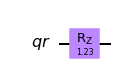
"""Example of using the Z gate."""
# Value of the external magenetic field.
h = 1.3 

# Display the circuit.
qr = QuantumRegister(1, "qr")
qc = QuantumCircuit(qr)
qc.rz(gamma * h * np.pi, qr)
qc.draw("mpl")

これらのゲートを行列にして、正しいかどうかを比較するパートはめんどくさいので省きました。

QiskitのRz(theta)ゲートとcirqのZ**(power)ゲートのちがい。

QiskitのRzゲートは、以下のように、指定するパラメタが"そのまま"行列要素における指数の肩に乗ります。

$$R Z(\lambda)=\exp \left(-i \frac{\lambda}{2} Z\right)=\left(\begin{array}{cc} e^{-i \frac{\lambda}{2}} & 0 \\ 0 & e^{i \frac{\lambda}{2}} \end{array}\right)$$

一方、CirqのZ**(power)は、そのパラメタに最初から$\pi$を含んだ形で行列の肩に乗ります。

$$R Z(\lambda)=\exp \left(-i \frac{\pi\lambda}{2} Z\right)=\left(\begin{array}{cc} e^{-i \frac{\pi\lambda}{2}} & 0 \\ 0 & e^{i \frac{\pi\lambda}{2}} \end{array}\right)$$

なので、QiskitとCirq間で翻訳するときはこの点に注意が必要です。

Implementing the full circuit

"""Define problem parameters and get a set of GridQubits."""
# Set the dimensions of the grid.
n_cols = 3
n_rows = 3

# Set the value of the external magnetic field at each site.
h = 0.5 * np.ones((n_rows, n_cols))

def gamma_layer(qc, qr, gamma_value, h):
    """Generator for U(gamma, C) layer of QAOA

    Args:
        gamma: Float variational parameter for the circuit
        h: Array of floats of external magnetic field values
    """
    for i in range(n_rows):
        for j in range(n_cols):
            if i < n_rows - 1:
                qc.rzz(gamma_value * np.pi, qr[i * n_cols + j], qr[(i + 1) * n_cols + j])
            if j < n_cols - 1:
                qc.rzz(gamma_value * np.pi, qr[i * n_cols + j], qr[i * n_cols + j + 1])
            qc.rz(gamma_value * h[i, j] * np.pi, qr[i * n_cols + j])

def beta_layer(qc, qr, beta_value):
    """Generator for U(beta, B) layer (mixing layer) of QAOA"""
    qc.rx(beta_value * np.pi, qr)

# edited
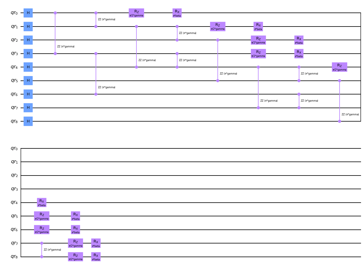
"""Create the QAOA circuit."""
# Use sympy.Symbols for the 𝛾 and β parameters.
gamma = Parameter("gamma")
beta = Parameter("beta")

qr = QuantumRegister(n_rows * n_cols, "qr")
qaoa = QuantumCircuit(qr, name="qaoa")

# Start in the H|0> state.
qaoa.h(qr)

# Implement the U(gamma, C) operator.
gamma_layer(qaoa, qr, gamma, h)

# Implement the U(beta, B) operator.
beta_layer(qaoa, qr, beta)

qaoa.draw("mpl")

Computing the energy

この部分は変えていません。

def energy_from_wavefunction(wf, h):
    """Computes the energy-per-site of the Ising model directly from the
    a given wavefunction. 

    Args:
        wf: Array of size 2**(n_rows * n_cols) specifying the wavefunction.
        h: Array of shape (n_rows, n_cols) giving the magnetic field values.

    Returns:
        energy: Float equal to the expectation value of the energy per site 
    """
    n_sites = n_rows * n_cols

    # Z is an array of shape (n_sites, 2**n_sites). Each row consists of the 
    # 2**n_sites non-zero entries in the operator that is the Pauli-Z matrix on
    # one of the qubits times the identities on the other qubits. The
    # (i*n_cols + j)th row corresponds to qubit (i,j).
    Z = np.array([(-1)**(np.arange(2**n_sites) >> i) for i in range(n_sites - 1, -1, -1)])

    # Create the operator corresponding to the interaction energy summed over all
    # nearest-neighbor pairs of qubits
    ZZ_filter = np.zeros_like(wf, dtype=float)
    for i in range(n_rows):
        for j in range(n_cols):
            if i < n_rows - 1:
                ZZ_filter += Z[i * n_cols + j] * Z[(i + 1) * n_cols + j]
            if j < n_cols - 1:
                ZZ_filter += Z[i * n_cols + j] * Z[i * n_cols + (j + 1)]

    energy_operator = -ZZ_filter - h.reshape(n_sites).dot(Z)

    # Expectation value of the energy divided by the number of sites
    return np.sum(np.abs(wf)**2 * energy_operator) / n_sites

上のenergy_from_wavefunction関数では、状態ベクトルを受け取ってエネルギーを計算しており、これは実際の量子デバイスでは使用できません。
代わりに、観測結果のhistogramからエネルギーを計算する方法を、以下に共有します。

def energy_from_hist(hist, h):
    """Computes the energy-per-site of the Ising model directly from the
    a given wavefunction. 

    Args:
        hist: Dictionary from str to int, specifying the measurement result.
        h: Array of shape (n_rows, n_cols) giving the magnetic field values.

    Returns:
        energy: Float equal to the expectation value of the energy per site 
    """
    n_sites = n_rows * n_cols
    shots = sum(list(hist.values()))
    
    h_expval = 0
    for site in range(n_sites):
        h_expval += h.reshape(n_sites)[site] * mit.expectation_value(reduce_hist(hist, [site]))[0]
    
    zz_expval = 0
    for i in range(n_rows):
        for j in range(n_cols):
            if i < n_rows - 1:
                zz_expval += mit.expectation_value(reduce_hist(hist, [i * n_cols + j]))[0] * mit.expectation_value(reduce_hist(hist, [(i + 1) * n_cols + j]))[0]
            if j < n_cols - 1:
                zz_expval += mit.expectation_value(reduce_hist(hist, [i * n_cols + j]))[0] * mit.expectation_value(reduce_hist(hist, [i * n_cols + (j + 1)]))[0]

    # Expectation value of the energy divided by the number of sites
    return (- zz_expval - h_expval) / n_sites

def energy_from_params(gamma_value, beta_value, qc, h):
    """Returns the energy given values of the parameters."""
    # backend = Aer.get_backend("qasm_simulator")
    backend = Aer.get_backend("statevector_simulator")
    
    bc = qc.bind_parameters({gamma: gamma_value, beta: beta_value})
    bc = bc.reverse_bits() # make statevector a little-endian form
    wf = execute(bc, backend=backend, optimization_level=0).result().get_statevector()
    return energy_from_wavefunction(wf, h)

Optimizing the parameters

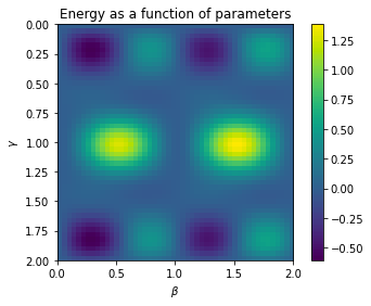
"""Do a grid search over values of 𝛄 and β."""
# Set the grid size and range of parameters.
grid_size = 50
gamma_max = 2
beta_max = 2

# Do the grid search.
energies = np.zeros((grid_size, grid_size))
for i in range(grid_size):
    for j in range(grid_size):
        energies[i, j] = energy_from_params(
            i * gamma_max / grid_size, j * beta_max / grid_size, qaoa, h
        )

"""Plot the energy as a function of the parameters 𝛄 and β found in the grid search."""
plt.ylabel(r"$\gamma$")
plt.xlabel(r"$\beta$")
plt.title("Energy as a function of parameters")
plt.imshow(energies, extent=(0, beta_max, gamma_max, 0))
plt.colorbar()
plt.show()

def gradient_energy(gamma, beta, qc, h):
    """Uses a symmetric difference to calulate the gradient."""
    eps = 10**-3 # Try different values of the discretization parameter

    # Gamma-component of the gradient
    grad_g = energy_from_params(gamma + eps, beta, qc, h)
    grad_g -= energy_from_params(gamma - eps, beta, qc, h)
    grad_g /= 2*eps

    # Beta-compoonent of the gradient
    grad_b = energy_from_params(gamma, beta + eps, qc, h)
    grad_b -= energy_from_params(gamma, beta - eps, qc, h)
    grad_b /= 2*eps  

    return grad_g, grad_b

"""Run a simple gradient descent optimizer."""
gamma_value, beta_value = 0.2, 0.7 # Try different initializations
eta = 10**-2 # Try adjusting the learning rate.

# Perform gradient descent for a given number of steps.
num_steps = 150
for i in range(num_steps + 1):
    # Compute the gradient.
    grad_g, grad_b = gradient_energy(gamma_value, beta_value, qaoa, h)

    # Update the parameters.
    gamma_value -= eta * grad_g
    beta_value -= eta * grad_b

    # Status updates.
    if not i % 25:
        print("Step: {} Energy: {}".format(i, energy_from_params(gamma_value, beta_value, qaoa, h)))

print("\nLearned gamma: {}\nLearned beta: {}".format(gamma_value, beta_value, qaoa, h))

Step: 0 Energy: 0.35551822054110027
Step: 25 Energy: -0.6065680507043341
Step: 50 Energy: -0.6068781774949847
Step: 75 Energy: -0.6068781801676347
Step: 100 Energy: -0.6068781801677109
Step: 125 Energy: -0.6068781801677107
Step: 150 Energy: -0.6068781801677109

Learned gamma: 0.19753237841096172
Learned beta: 0.2684381345958432

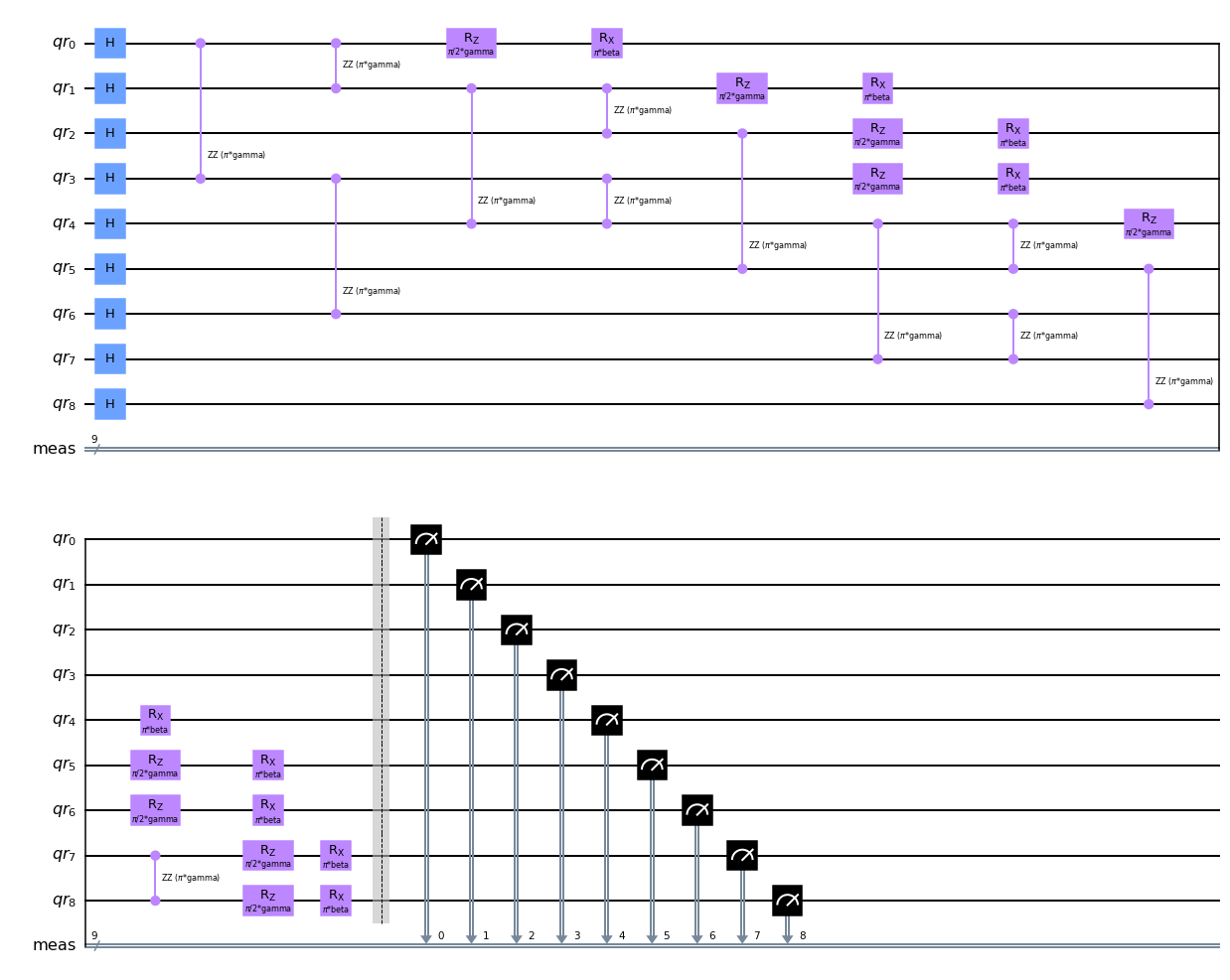
Getting the approximate solutions

"""Add measurements to the QAOA circuit."""
qaoa_meas = qaoa.copy()
qaoa_meas.measure_all()
qaoa_meas.draw("mpl")

"""Sample from the QAOA circuit."""
num_reps = 1000  # Try different numbers of repetitions.
gamma_value, beta_value = 0.2, 0.25  # Try different values of the parameters.

# Sample from the circuit.
backend = Aer.get_backend("qasm_simulator")
bc = qaoa_meas.bind_parameters({gamma: gamma_value, beta: beta_value})
bc = bc.reverse_bits() # make statevector a little-endian form
result = execute(bc, backend=backend, shots=num_reps, optimization_level=0).result()

def compute_energy(meas):
    """Returns the energy computed from measurements.

    Args:
        meas: Measurements/samples.
    """
    Z_vals = 1 - 2 * meas.reshape(n_rows,n_cols)
    energy = 0
    for i in range(n_rows):
        for j in range(n_cols):
            if i < n_rows - 1:
                energy -= Z_vals[i, j] * Z_vals[i + 1, j]
            if j < n_cols - 1:
                energy -= Z_vals[i, j] * Z_vals[i, j + 1]
            energy -= h[i, j] * Z_vals[i, j]
    return energy / (n_rows * n_cols)

"""Compute the energies of the most common measurement results."""
# Get a histogram of the measurement results.
hist = result.get_counts()

# Consider the top 10 of them.
num = 10

# Get the most common measurement results and their probabilities.
configs = [int(k, 2) for k, v in sorted(hist.items(), key=lambda item: -item[1])[:num]]
probs = [v / num_reps for k, v in sorted(hist.items(), key=lambda item: -item[1])[:num]]

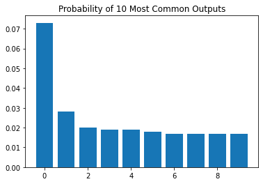
"""Plot the most common measurement results and their energies."""
# Plot probabilities of the most common bitstrings.
plt.title("Probability of {} Most Common Outputs".format(num))
plt.bar([x for x in range(len(probs))],probs)
plt.show()
meas = [[int(s) for s in "".join([str(b) for b in bin(k)[2:]]).zfill(n_rows * n_cols)] for k in configs]
costs = [compute_energy(np.array(m)) for m in meas]

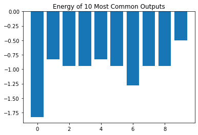
# Plot energies of the most common bitstrings.
plt.title("Energy of {} Most Common Outputs".format(num))
plt.bar([x for x in range(len(costs))], costs)
plt.show()
print("Fraction of outputs displayed: {}".format(np.sum(probs).round(2)))

Fraction of outputs displayed: 0.24