🐷

一致性と不偏性③

2024/05/03に公開

Python

統計

tech

3行まとめ

一致性と不偏性を実際に試してみました
正規分布、ポワソン分布に加えて、適当な母集団についても実験しました
やっぱりコードを書いて結果が出てくるのは楽しいね

参考書籍

入門詐欺として有名な統計学入門を使って勉強しています。
https://amzn.to/4dmDECE

前回のあらすじ

前回の3行要約

よく問われる標本分散の不偏性は母分散と平均の分散の形にうまく持っていくと証明できる
一致性はシェビチェフの不等式に持っていって、 $n \to \infty$ の時の期待値と分散に着目
シェビチェフの不等式はすごい

今回は、一致性と不偏性の締めくくりとして、母平均と母分散を設定した上で実際にpythonで乱数を発生させて遊んでみました。

実験の概要

ここまでの議論では母集団分布の種類を限定しておらず、標本平均と不偏分散の一致性、不偏性の証明でも、特に母集団分布が〇〇である、という仮定はしいていませんでした。
そこで、今回の実験では以下の3つの母集団を準備します。

正規分布に従う母集団
ポワソン分布に従う母集団
ガンマ分布とベータ分布をランダムに組み合わせて作成したノンパラメトリックな母集団

それぞれの分布について、以下の３ステップで実験を行なっていきます。

母集団分布の可視化
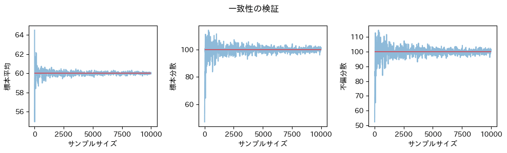
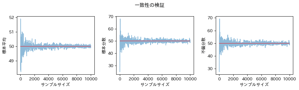
一致性の確認
サンプルサイズを10~10,000で10刻みに増加させていき、それぞれのサンプルから推定量を計算します。
サンプルサイズが大きくなったとき、推定量は果たして母数に一致するか？ということを確かめます。
不偏性の確認
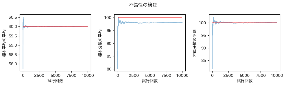
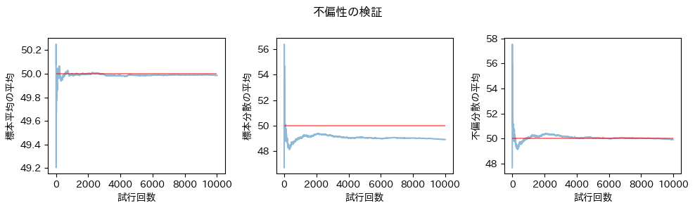
サンプルサイズは一定(50としました)として、そのサンプリング行為自体を増やしていきます(1~10,000回としました)。
推定量がどんどん得られていくにつれて、それらの平均値は果たして母数に一致するか？ということを確かめます。

なお、今回ターゲットとする推定量は、標本平均、標本分散、不偏分散の3つとします。

コードに関して

以下、実験や製図に使用したコードをトグルにて記述します。
python3.10.11でjupyter notebook上で実施していますが、大したコードではないので細かいパッケージのバージョン情報は割愛します。
また、すべて冒頭で以下のパッケージ、ライブラリをインポートしていることが前提で記載しています。

import numpy as np
import scipy.stats as st
import matplotlib.pyplot as plt
import os
import japanize_matplotlib.japanize_matplotlib

SEED = 42
SAVE_DIR = '任意のディレクトリ'

結果

正規分布に従う母集団

母集団分布

正規母集団の可視化

コード

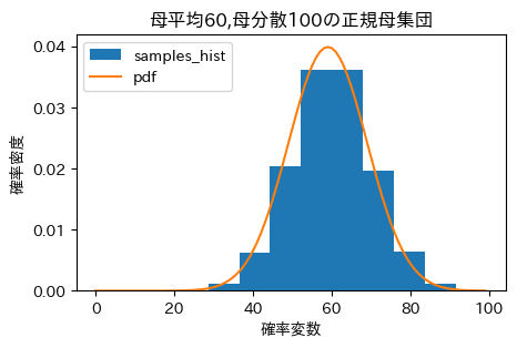
mu = 60 # 母平均の設定
sigma_2 = 10**2 # 母分散の設定
np.random.seed(SEED)
sample = np.random.normal(
 loc=mu,
 scale=np.sqrt(sigma_2),
 size=10000,
 )

plt.figure(figsize=(5,3))

plt.hist(
 sample,
 density=True,
 label='samples_hist',
 )

p = st.norm.pdf(
 x=np.arange(1,101,1),
 loc = mu,
 scale =np.sqrt(sigma_2),
)
plt.plot(p,label='pdf')
plt.legend(loc='best')
plt.xlabel('確率変数')
plt.ylabel('確率密度')
plt.title(f'母平均{mu},母分散{sigma_2}の正規母集団')
plt.savefig(f'{SAVE_DIR}/正規母集団.png',bbox_inches='tight')
plt.show()

実践は密度関数を、ヒストグラムは10,000個発生させた乱数の分布を示していますが、綺麗なベルカーブが見れますね。

一致性の確認

コード

mu = 60 # 母平均の設定
sigma_2 = 10**2 # 母分散の設定
np.random.seed(SEED)

# サンプルサイズは10~10,000を10刻み
sample_size = np.arange(10,10001,10)

x_bar = np.zeros(len(sample_size))
S_2 = np.zeros(len(sample_size))
s_2 = np.zeros(len(sample_size))

for size in sample_size:
 sample = np.random.normal(
  loc=mu,
  scale=np.sqrt(sigma_2),
  size=size,
  )
 x_bar[sample_size==size]=np.mean(sample)
 S_2[sample_size==size]=np.var(sample,ddof=0)
 s_2[sample_size==size]=np.var(sample,ddof=1)
fig, axes = plt.subplots(
 ncols=3,
 nrows=1,
 figsize=(10,3),
 tight_layout=True,
)

for ax,score,answer,title in zip(
 axes,
 [x_bar,S_2,s_2],
 [mu,sigma_2,sigma_2],
 ['標本平均','標本分散','不偏分散']
 ):
 ax.plot(
  sample_size,
  score,
  alpha=.5,
 )
 ax.hlines(
  xmin=0,
  xmax=np.max(sample_size),
  y=answer,
  alpha=0.5,
  colors='r',
 )
 ax.set_xlabel('サンプルサイズ')
 ax.set_ylabel(title)
fig.suptitle('一致性の検証')
plt.savefig(f'{SAVE_DIR}/正規母集団_一致性.png',bbox_inches='tight')
plt.show()

証明通り^[1]、3つの推定量はすべてサンプルサイズを極大にしたときに母数に収束しそうな雰囲気が感じられます。

不偏性の確認

不偏性

コード

mu = 60 # 母平均の設定
sigma_2 = 10**2 # 母分散の設定
sample_size = 50 # サンプルサイズは100
trial = 10000 # 試行回数を3000回
np.random.seed(SEED)

# 各試行で得られる推定量を格納するリスト
x_bar = []
S_2 = []
s_2 = []

# 各試行終了時の推定量の平均を格納するリスト
mean_x_bar = []
mean_S_2 = []
mean_s_2 = []

for i in range(trial):
 sample = np.random.normal(
  loc=mu,
  scale=np.sqrt(sigma_2),
  size=sample_size
  )
 x_bar.append(np.mean(sample))
 mean_x_bar.append(np.mean(x_bar))
 S_2.append(np.var(sample,ddof=0))
 mean_S_2.append(np.mean(S_2))
 s_2.append(np.var(sample,ddof=1))
 mean_s_2.append(np.mean(s_2))
fig, axes = plt.subplots(
 ncols=3,
 nrows=1,
 figsize=(10,3),
 tight_layout=True,
)

for ax,score,answer,title in zip(
 axes,
 # [x_bar,S_2,s_2],
 [mean_x_bar,mean_S_2,mean_s_2],
 [mu,sigma_2,sigma_2],
 ['標本平均','標本分散','不偏分散']
 ):
 ax.plot(
  np.arange(trial)+1,
  score,
  alpha=.5,
 )
 ax.hlines(
  xmin=0,
  xmax=trial,
  y=answer,
  alpha=0.5,
  colors='r',
 )
 ax.set_xlabel('試行回数')
 ax.set_ylabel(f'{title}の平均')
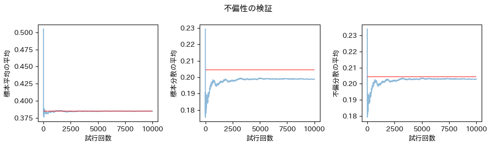
fig.suptitle('不偏性の検証')
plt.savefig(f'{SAVE_DIR}/正規母集団_不偏性.png',bbox_inches='tight')
plt.show()

「おぉ！やっぱり標本分散はアカンのや！」
となる結果が得られましたね。
証明通り標本分散は、真の分散と比べて低く見積もられがち、というところが如実に現れています。

ポワソン分布に従う母集団

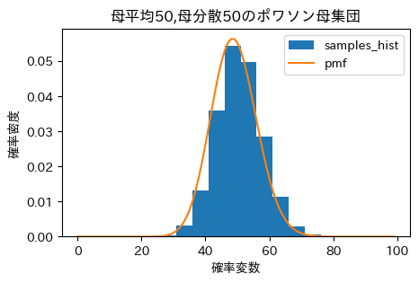
ポワソン分布は、以下の確率質量関数で表される離散確率分布であり、確率変数が正の整数であることを前提としているため、回数とか個数みたいな事柄に関連する確率を考える際に採用されがち^[2]です。

P(X=x)=\frac{\lambda^x}{x!}e^{-\lambda} \quad \footnotesize x=\{0,1,2,3,\dots\}

この分布は平均と分散がどちらも $\lambda$ になり^[3]、これに対する推定量の一致性と不偏性を確かめていきます。
サクッといきます。

母集団分布

ポワソン分布

コード

lam = 50 # パラメータ設定
np.random.seed(SEED)
sample = np.random.poisson(
 lam=lam,
 size=10000,
 )

plt.figure(figsize=(5,3))

plt.hist(
 sample,
 density=True,
 label='samples_hist',
 )

p = st.poisson.pmf(
 k=np.arange(1,101,1),
 mu=lam
)
plt.plot(p,label='pmf')
plt.legend(loc='best')
plt.xlabel('確率変数')
plt.ylabel('確率密度')
plt.title(f'母平均{lam},母分散{lam}のポワソン母集団')
plt.savefig(f'{SAVE_DIR}/ポワソン母集団.png',bbox_inches='tight')
plt.show()

一致性の確認

一致性

コード

np.random.seed(SEED)

# サンプルサイズは10~10,000を10刻み
sample_size = np.arange(10,10001,10)

x_bar = np.zeros(len(sample_size))
S_2 = np.zeros(len(sample_size))
s_2 = np.zeros(len(sample_size))

for size in sample_size:
 sample = np.random.poisson(
  lam=lam,
  size=size,
  )
 x_bar[sample_size==size]=np.mean(sample)
 S_2[sample_size==size]=np.var(sample,ddof=0)
 s_2[sample_size==size]=np.var(sample,ddof=1)
fig, axes = plt.subplots(
 ncols=3,
 nrows=1,
 figsize=(10,3),
 tight_layout=True,
)

for ax,score,answer,title in zip(
 axes,
 [x_bar,S_2,s_2],
 [lam,lam,lam],
 ['標本平均','標本分散','不偏分散']
 ):
 ax.plot(
  sample_size,
  score,
  alpha=.5,
 )
 ax.hlines(
  xmin=0,
  xmax=np.max(sample_size),
  y=answer,
  alpha=0.5,
  colors='r',
 )
 ax.set_xlabel('サンプルサイズ')
 ax.set_ylabel(title)
fig.suptitle('一致性の検証')
plt.savefig(f'{SAVE_DIR}/ポワソン母集団_一致性.png',bbox_inches='tight')
plt.show()

不偏性の確認

不偏性

コード

sample_size = 50 # サンプルサイズは100
trial = 10000 # 試行回数を3000回
np.random.seed(SEED)

# 各試行で得られる推定量を格納するリスト
x_bar = []
S_2 = []
s_2 = []

# 各試行終了時の推定量の平均を格納するリスト
mean_x_bar = []
mean_S_2 = []
mean_s_2 = []

for i in range(trial):
 sample = np.random.poisson(
  lam=lam,
  size=sample_size,
  )
 x_bar.append(np.mean(sample))
 mean_x_bar.append(np.mean(x_bar))
 S_2.append(np.var(sample,ddof=0))
 mean_S_2.append(np.mean(S_2))
 s_2.append(np.var(sample,ddof=1))
 mean_s_2.append(np.mean(s_2))
fig, axes = plt.subplots(
 ncols=3,
 nrows=1,
 figsize=(10,3),
 tight_layout=True,
)

for ax,score,answer,title in zip(
 axes,
 # [x_bar,S_2,s_2],
 [mean_x_bar,mean_S_2,mean_s_2],
 [lam,lam,lam],
 ['標本平均','標本分散','不偏分散']
 ):
 ax.plot(
  np.arange(trial)+1,
  score,
  alpha=.5,
 )
 ax.hlines(
  xmin=0,
  xmax=trial,
  y=answer,
  alpha=0.5,
  colors='r',
 )
 ax.set_xlabel('試行回数')
 ax.set_ylabel(f'{title}の平均')
fig.suptitle('不偏性の検証')
plt.savefig(f'{SAVE_DIR}/ポワソン母集団_不偏性.png',bbox_inches='tight')
plt.show()

なんべんやっても、標本分散に不偏性がないことがビジュアルとして出てくる瞬間はキモティイィイイィィイイィ！！！

ノンパラメトリック

例えば二峰性があったり、明らかに複数のパラメトリックな分布が重複して効いていそうなごちゃっとした分布に対しても成り立つのでしょうか？
ということで、作った本人でさえもパラメトリックに再現することができない分布として、パラメータをランダムに指定したガンマ分布orベータ分布を100個用意して、そこから1,000個ずつサンプリングして得られた100,000個の数値を母集団とした実験をしてみました。

母集団分布

ノンパラ

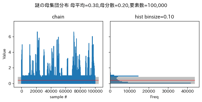
なんだかうまくいってない時のMCMCサンプリング結果みたいな、いい感じの分布が得られましたよ。

コード

# 乱数ジェネレータのインスタンス作成
rvg = np.random.default_rng()

np.random.seed(SEED)

# ガンマ分布がベータ分布かのどちらかをランダムに選び、
# ランダムに決められたパラメータに基づいて1,000個の乱数を取得、
# という操作を100回繰り返して、ノンパラメトリックな100,000個の
# 数値からなる母集団を作成する。

kinds = [
    rvg.gamma,
    rvg.beta
    ]
each_size = 1000
iter = 100
population=[]

for i in range(iter):
 arg1,arg2 = np.random.rand(2)
 gen = np.random.choice(kinds)
 samples = gen(arg1,arg2,each_size)
 population.append(samples)
population = np.array(population).ravel()

fig,axes = plt.subplots(
 1,2,
 figsize=(7,3.5),
 tight_layout=True,
 sharey=True
)

axes[0].plot(population)
axes[0].set_xlabel('sample #')
axes[0].set_ylabel('Value')
axes[0].set_title('chain')

binwidth = .1
bins=np.arange(np.min(population),np.max(population)+1,binwidth)
axes[1].hist(population,bins=bins,orientation='horizontal')
axes[1].set_xlabel('Freq')
axes[1].set_title(f'hist binsize={binwidth:.2f}')

mu = np.mean(population)
sigma_2 = np.var(population,ddof=0)

for ax in axes:
 xmin,xmax = ax.get_xlim()
 ax.hlines(xmin=xmin,xmax=xmax,y=mu,colors='red',alpha=.5)
 ax.fill_between(
  x=np.linspace(xmin,xmax,1000),
  y1=mu-np.sqrt(sigma_2),
  y2=mu+np.sqrt(sigma_2),
  facecolor='gray',
  alpha=.5
  )

fig.suptitle(f'謎の母集団分布 母平均={mu:.2f},母分散={sigma_2:.2f},要素数={len(population):,}')
plt.savefig(f'{SAVE_DIR}/ノンパラ母集団.png',bbox_inches='tight')
plt.show()

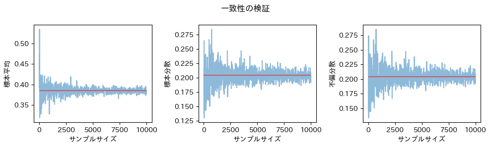
一致性の確認

一致性

コード

np.random.seed(SEED)

# サンプルサイズは10~10,000を10刻み
sample_size = np.arange(10,10001,10)

x_bar = np.zeros(len(sample_size))
S_2 = np.zeros(len(sample_size))
s_2 = np.zeros(len(sample_size))

for size in sample_size:
 sample = np.random.choice(
  population,
  size=size,
  )
 x_bar[sample_size==size]=np.mean(sample)
 S_2[sample_size==size]=np.var(sample,ddof=0)
 s_2[sample_size==size]=np.var(sample,ddof=1)
fig, axes = plt.subplots(
 ncols=3,
 nrows=1,
 figsize=(10,3),
 tight_layout=True,
)

for ax,score,answer,title in zip(
 axes,
 [x_bar,S_2,s_2],
 [mu,sigma_2,sigma_2],
 ['標本平均','標本分散','不偏分散']
 ):
 ax.plot(
  sample_size,
  score,
  alpha=.5,
 )
 ax.hlines(
  xmin=0,
  xmax=np.max(sample_size),
  y=answer,
  alpha=0.5,
  colors='r',
 )
 ax.set_xlabel('サンプルサイズ')
 ax.set_ylabel(title)
fig.suptitle('一致性の検証')
plt.savefig(f'{SAVE_DIR}/ノンパラ母集団_一致性.png',bbox_inches='tight')
plt.show()

単峰性と比べると、サンプリング結果のばらつきが大きいので、収束するまでに必要なサンプル数は増える傾向にありますが、なんとなく母数に収束しそうな感じです。

不偏性の確認

不偏性

コード

sample_size = 50 # サンプルサイズは100
trial = 10000 # 試行回数を3000回
np.random.seed(SEED)

# 各試行で得られる推定量を格納するリスト
x_bar = []
S_2 = []
s_2 = []

# 各試行終了時の推定量の平均を格納するリスト
mean_x_bar = []
mean_S_2 = []
mean_s_2 = []

for i in range(trial):
 sample = np.random.choice(
  population,
  size=sample_size
  )
 x_bar.append(np.mean(sample))
 mean_x_bar.append(np.mean(x_bar))
 S_2.append(np.var(sample,ddof=0))
 mean_S_2.append(np.mean(S_2))
 s_2.append(np.var(sample,ddof=1))
 mean_s_2.append(np.mean(s_2))
fig, axes = plt.subplots(
 ncols=3,
 nrows=1,
 figsize=(10,3),
 tight_layout=True,
)

for ax,score,answer,title in zip(
 axes,
 # [x_bar,S_2,s_2],
 [mean_x_bar,mean_S_2,mean_s_2],
 [mu,sigma_2,sigma_2],
 ['標本平均','標本分散','不偏分散']
 ):
 ax.plot(
  np.arange(trial)+1,
  score,
  alpha=.5,
 )
 ax.hlines(
  xmin=0,
  xmax=trial,
  y=answer,
  alpha=0.5,
  colors='r',
 )
 ax.set_xlabel('試行回数')
 ax.set_ylabel(f'{title}の平均')
fig.suptitle('不偏性の検証')
plt.savefig(f'{SAVE_DIR}/ノンパラ母集団_不偏性.png',bbox_inches='tight')
plt.show()

ンギモティイィイィイィイィイィイィイィイィイィイィイイイィイ！！！！
こちらもやはり単峰性と比べると、サンプリング結果のばらつきが大きいので、収束するまでに必要な試行数は増える傾向にありますが、ノンパラメトリックでもしっかりと不偏分散に不偏性があることが確かめれらましたね！

終わりに

やっぱりコードを書いて、想定された結果が綺麗に図示された瞬間、たまらないですね！
うっかり3回に跨ってしまいましたが、不偏性、一致性について理解がある程度定着したような気がします。
単純にここの単元だけ読んでいても、ふんふんとわかった気になってしまうのですが、最小二乗推定量がBLUEであること、みたいなところで突然出てきて、あれあれ〜となってしまいがち。
次は最小二乗法についてもきちんと復習したいなあという所存です。

以上、ご確認のほど、よろしくお願いいたします。

脚注

厳密にいうと標本分散、不偏分散の一致性の証明はサボりました。 ↩︎
実際のところは、単位時間あたりに平均 $\lambda$ 回発生する事象が、次の単位時間内に発生する回数Xが従う確率分布、です。 ↩︎
なので、標本平均と不偏分散が大体同じくらいになってないと、ほんとにポワソン分布でフィッティングしても良いのか？ということになりますね。 ↩︎

GitHubで編集を提案

3行まとめ

参考書籍

前回のあらすじ

実験の概要

結果

正規分布に従う母集団

母集団分布

一致性の確認

不偏性の確認

ポワソン分布に従う母集団

母集団分布

一致性の確認

不偏性の確認

ノンパラメトリック

母集団分布

一致性の確認

不偏性の確認

終わりに

Discussion