光学衛星画像から位置情報埋め込みの基盤モデル SatCLIP の実装と使い方
近年、衛星利用の動きは、日々発展しています。コンピュータービジョンでの応用は特に、展開が早いです。

https://github.com/microsoft/satclip/blob/main/figures/globes.gif より引用
そんな中、位置情報とも関連する衛星データ処理にも変革が訪れつつあるので、その一例をご紹介します。
SatCLIP
今回はご紹介するのは SatCLIP とモデルであり、手法の提案です。
公式リンク
Microsoft が論文と共にコードもオープンソースで公開しています。
Github:
Paper:
概要
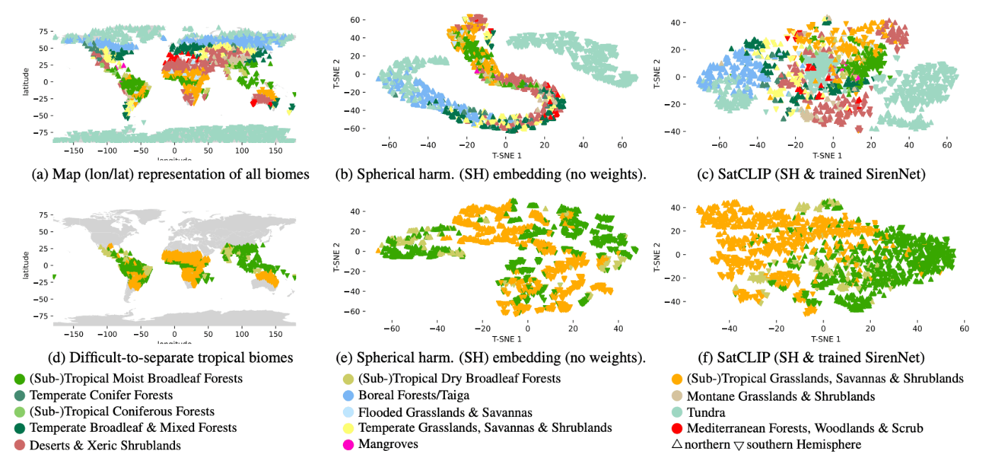
ビジョントランスフォーマー(Vision Transformer)と CLIP を使用して位置情報を LLM の基盤モデルに置き換えたマルチモーダルによる提案です。
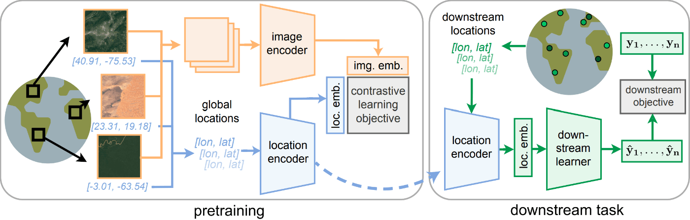
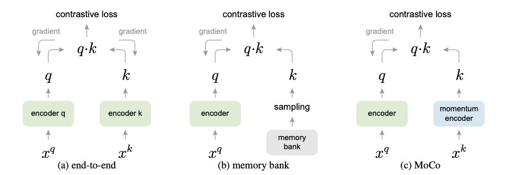
学習の手法は教師なし学習で、自己を教師としてモーメントをかけた特徴量を自身と一致させるような MOCO という contrastive learning の1つの方法を用いています。これによって画像の埋め込みを取得します。
それに対して、CLIP の基盤モデルの使用方法と同じように、画像の埋め込みと位置情報の埋め込み ( img. emb. と loc. emb. ) が近くなるように location encoder を学習させます。
学習データは Microsft の Planetary Computer の Sentinel-2 L2A です。
使用方法
例 1
SatCLIP の位置情報の埋め込みを取得する例です。
まずは、上部でインストールを行います。
!wget 'https://satclip.z13.web.core.windows.net/satclip/satclip-resnet18-l10.ckpt'
こちらで学習済みモデルを取得します。
import sys
sys.path.append('./satclip')

import torch
from load import get_satclip
こちらでインポートをします。
satclip_path = 'satclip-resnet18-l10.ckpt'

device = torch.device('cuda' if torch.cuda.is_available() else 'cpu')

c = torch.randn(32, 2) # Represents a batch of 32 locations (lon/lat)

model = get_satclip(satclip_path, device=device) # Only loads location encoder by default
model.eval()
with torch.no_grad():
  emb  = model(c.double().to(device)).detach().cpu()
ここでは、サンプルの c の緯度経度に対して、 SatCLIP の埋め込み情報を取得しています。
この emb が全球を考慮した、グローバルな意味的位置情報になります。
AI によって生成された潜在的な位置情報ですね。
例 2
こちらでは、生成された潜在的な位置情報 は位置を反映しているはずなので、温度も自然と赤道の近さから予測できるという過程の確認のために、モデルを学習と予測して実験しています。
上部はインストールと基本的に例1と同じなので割愛します。
はじめに、気温のデータセットを取得します。
from urllib import request
import numpy as np
import pandas as pd
import io
import torch


def get_air_temp_data(pred="temp",norm_y=True,norm_x=True):
  '''
  Download and process the Global Air Temperature dataset (more info: https://www.nature.com/articles/sdata2018246)

  Parameters:
  pred = numeric; outcome variable to be returned; choose from ["temp", "prec"]
  norm_y = logical; should outcome be normalized
  norm_min_val = integer; choice of [0,1], setting whether normalization in range[0,1] or [-1,1]

  Return:
  coords = spatial coordinates (lon/lat)
  x = features at location
  y = outcome variable
  '''
  url = 'https://springernature.figshare.com/ndownloader/files/12609182'
  url_open = request.urlopen(url)
  inc = np.array(pd.read_csv(io.StringIO(url_open.read().decode('utf-8'))))
  coords = inc[:,:2]
  if pred=="temp":
    y = inc[:,4].reshape(-1)
    x = inc[:,5]
  else:
    y = inc[:,5].reshape(-1)
    x = inc[:,4]
  if norm_y==True:
    y = y / y.max()
  if norm_x==True:
    x = x / x.max()

  return torch.tensor(coords), torch.tensor(x), torch.tensor(y)

coords, _, y = get_air_temp_data()

import matplotlib.pyplot as plt
from mpl_toolkits.basemap import Basemap

fig, ax = plt.subplots(1, figsize=(5, 3))

m = Basemap(projection='cyl', resolution='c', ax=ax)
m.drawcoastlines()
ax.scatter(coords[:,0], coords[:,1], c=y, s=5)
ax.set_title('Annual Mean Temperatures')
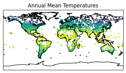
なんとなくですが、極地から赤道まで色のグラデーションになってい事がわかると思います。
satclip_path = 'satclip-vit16-l10.ckpt'
model = get_satclip(satclip_path, device=device) # Only loads location encoder by default
model.eval()
with torch.no_grad():
x = model(coords.double().to(device)).detach().cpu()
from torch.utils.data import TensorDataset, random_split
dataset = TensorDataset(coords, x, y)
train_size = int(0.5 * len(dataset))
test_size = len(dataset) - train_size
train_set, test_set = random_split(dataset, [train_size, test_size])
coords_train, x_train, y_train = train_set.dataset.tensors[0][train_set.indices], train_set.dataset.tensors[1][train_set.indices], train_set.dataset.tensors[2][train_set.indices]
coords_test, x_test, y_test = test_set.dataset.tensors[0][test_set.indices], test_set.dataset.tensors[1][test_set.indices], test_set.dataset.tensors[2][test_set.indices]
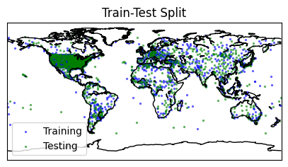
fig, ax = plt.subplots(1, figsize=(5, 3))
m = Basemap(projection='cyl', resolution='c', ax=ax)
m.drawcoastlines()
ax.scatter(coords_train[:,0], coords_train[:,1], c='blue', s=2, label='Training',alpha=0.5)
ax.scatter(coords_test[:,0], coords_test[:,1], c='green', s=2, label='Testing',alpha=0.5)
ax.legend()
ax.set_title('Train-Test Split')
それぞれの位置情報から埋め込みを取得して、学習と検証に分割します。
import torch.nn as nn

class MLP(nn.Module):
    def __init__(self, input_dim, dim_hidden, num_layers, out_dims):
        super(MLP, self).__init__()

        layers = []
        layers += [nn.Linear(input_dim, dim_hidden, bias=True), nn.ReLU()] # Input layer
        layers += [nn.Linear(dim_hidden, dim_hidden, bias=True), nn.ReLU()] * num_layers # Hidden layers
        layers += [nn.Linear(dim_hidden, out_dims, bias=True)] # Output layer

        self.features = nn.Sequential(*layers)

    def forward(self, x):
        return self.features(x)

pred_model = MLP(input_dim=256, dim_hidden=64, num_layers=2, out_dims=1).float().to(device)
criterion = nn.MSELoss()
optimizer = torch.optim.Adam(pred_model.parameters(), lr=0.001)

losses = []
epochs = 3000

for epoch in range(epochs):
  optimizer.zero_grad()
  # Forward pass
  y_pred = pred_model(x_train.float().to(device))
  # Compute the loss
  loss = criterion(y_pred.reshape(-1), y_train.float().to(device))
  # Backward pass
  loss.backward()
  # Update the parameters
  optimizer.step()
  # Append the loss to the list
  losses.append(loss.item())
  if (epoch + 1) % 250 == 0:
    print(f"Epoch {epoch + 1}, Loss: {loss.item():.4f}")
簡単なモデルを定義して埋め込みから気温を学習させます。
with torch.no_grad():
  model.eval()
  y_pred_test = pred_model(x_test.float().to(device))

# Print test loss
print(f'Test loss: {criterion(y_pred_test.reshape(-1), y_test.float().to(device)).item()}')

fig, ax = plt.subplots(1, 2, figsize=(10, 3))

m = Basemap(projection='cyl', resolution='c', ax=ax[0])
m.drawcoastlines()
ax[0].scatter(coords_test[:,0], coords_test[:,1], c=y_test, s=5)
ax[0].set_title('True')

m = Basemap(projection='cyl', resolution='c', ax=ax[1])
m.drawcoastlines()
ax[1].scatter(coords_test[:,0], coords_test[:,1], c=y_pred_test.reshape(-1), s=5)
ax[1].set_title('Predicted')
最後に検証データで予測をします。
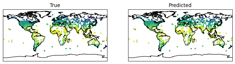
だいたい、学習も検証も遜色ないような定性評価ができると思います。
ということは、AI によって生成された潜在的な位置情報 は確からしいということが少しは示そうですね。
実用例と実装
Sentinel-Hub
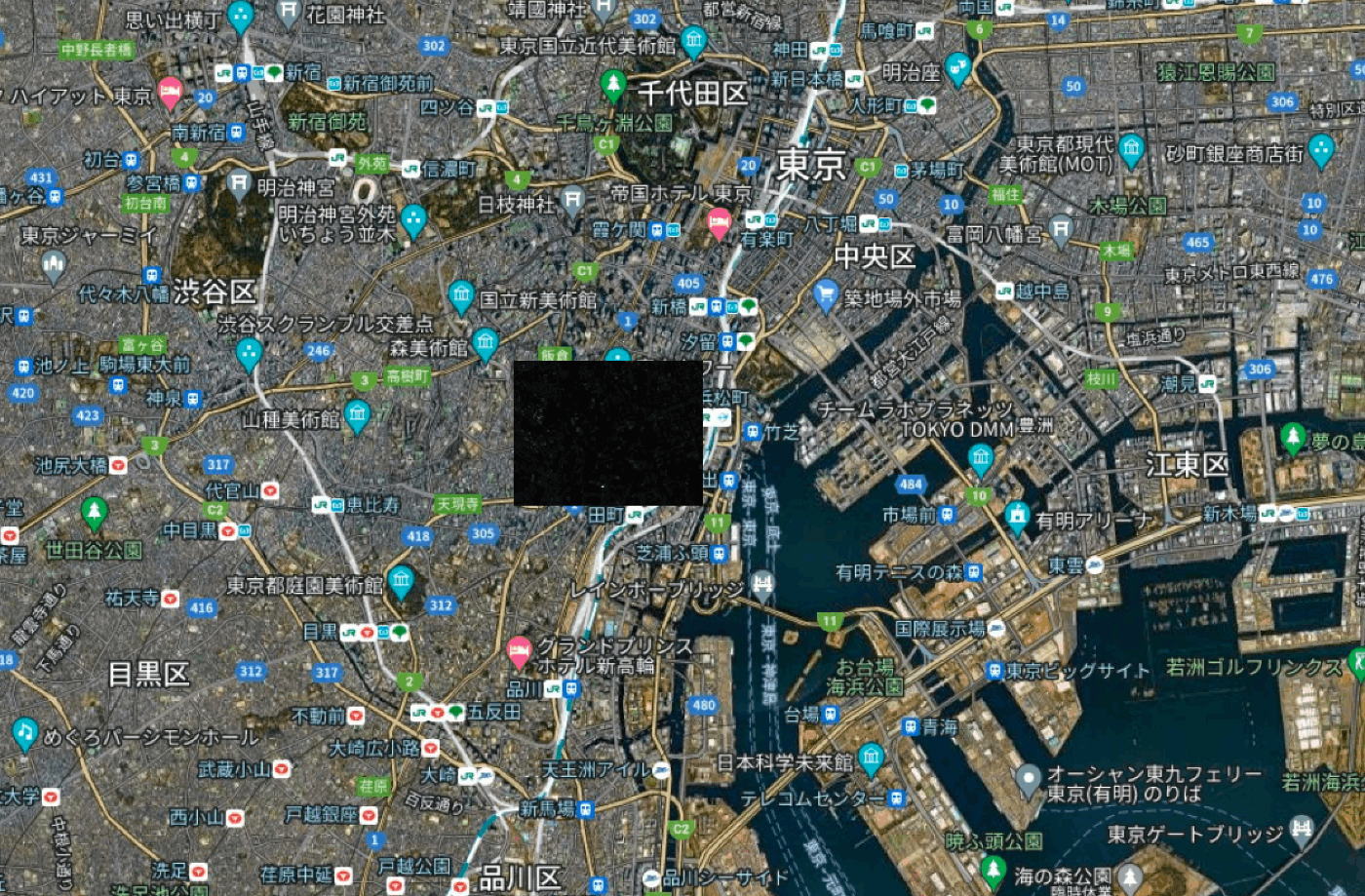
東京の港区エリアをターゲットにします。
AWS の S3 ストレージからデータを取得します。
aws s3 cp s3://sentinel-s2-l2a/tiles/54/S/UE/2023/12/8/0/ ./Desktop/ --recursive --request-payer requester
ターゲットの座標は以下です。
- 左上:
139.727043,35.671531 - 右下:
139.755838,35.661023
この情報でくり抜く場合は
gdalwarp -te 139.727043 35.639720 139.756399 35.671531 -t_srs EPSG:4326 R10m/B02.jp2 R10m/B02_crop.jp2
詳しい切り出しについては以前、私が執筆した以下の記事が詳しいです。
以下は同一作業です。
# Resolution 10m
gdalwarp -te 139.727043 35.639720 139.756399 35.671531 -t_srs EPSG:4326 R10m/B03.jp2 R10m/B03_crop.jp2
gdalwarp -te 139.727043 35.639720 139.756399 35.671531 -t_srs EPSG:4326 R10m/B04.jp2 R10m/B04_crop.jp2
gdalwarp -te 139.727043 35.639720 139.756399 35.671531 -t_srs EPSG:4326 R10m/B08.jp2 R10m/B08_crop.jp2

# Resolution 20m
gdalwarp -te 139.727043 35.639720 139.756399 35.671531 -t_srs EPSG:4326 R20m/B01.jp2 R20m/B01_crop.jp2
gdalwarp -te 139.727043 35.639720 139.756399 35.671531 -t_srs EPSG:4326 R20m/B05.jp2 R20m/B05_crop.jp2
gdalwarp -te 139.727043 35.639720 139.756399 35.671531 -t_srs EPSG:4326 R20m/B06.jp2 R20m/B06_crop.jp2
gdalwarp -te 139.727043 35.639720 139.756399 35.671531 -t_srs EPSG:4326 R20m/B07.jp2 R20m/B07_crop.jp2
gdalwarp -te 139.727043 35.639720 139.756399 35.671531 -t_srs EPSG:4326 R20m/B8A.jp2 R20m/B8A_crop.jp2
gdalwarp -te 139.727043 35.639720 139.756399 35.671531 -t_srs EPSG:4326 R20m/B11.jp2 R20m/B11_crop.jp2
gdalwarp -te 139.727043 35.639720 139.756399 35.671531 -t_srs EPSG:4326 R20m/B12.jp2 R20m/B12_crop.jp2

# Resolution 60m
gdalwarp -te 139.727043 35.639720 139.756399 35.671531 -t_srs EPSG:4326 R60m/B09.jp2 R60m/B09_crop.jp2
Gdal のコマンドを利用して組み合わせます。
実際に、画像をレイヤーとして積み上げます。
gdal_merge.py -ps 0.0001001911262797905151 -0.000100350157728721441 -separate R20m/B01_crop.jp2 R10m/B02_crop.jp2 R10m/B03_crop.jp2 R10m/B04_crop.jp2 R20m/B05_crop.jp2 R20m/B06_crop.jp2 R20m/B06_crop.jp2 R20m/B07_crop.jp2 R10m/B08_crop.jp2 R20m/B8A_crop.jp2 R60m/B09_crop.jp2 R20m/B11_crop.jp2 R20m/B12_crop.jp2 -o merge.tif
注意点としては 10m 解像度に -ps で統一させています。
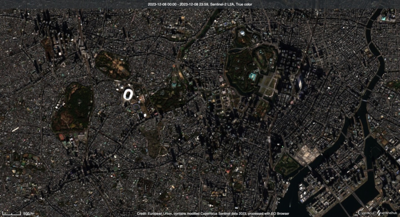
可視化します。
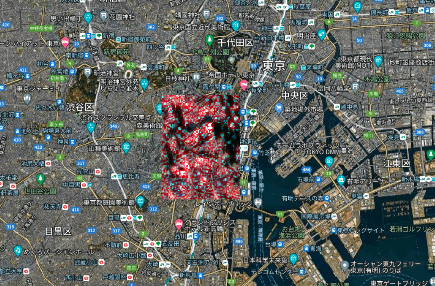
バンドの最初の3バンドのみを可視化しています。
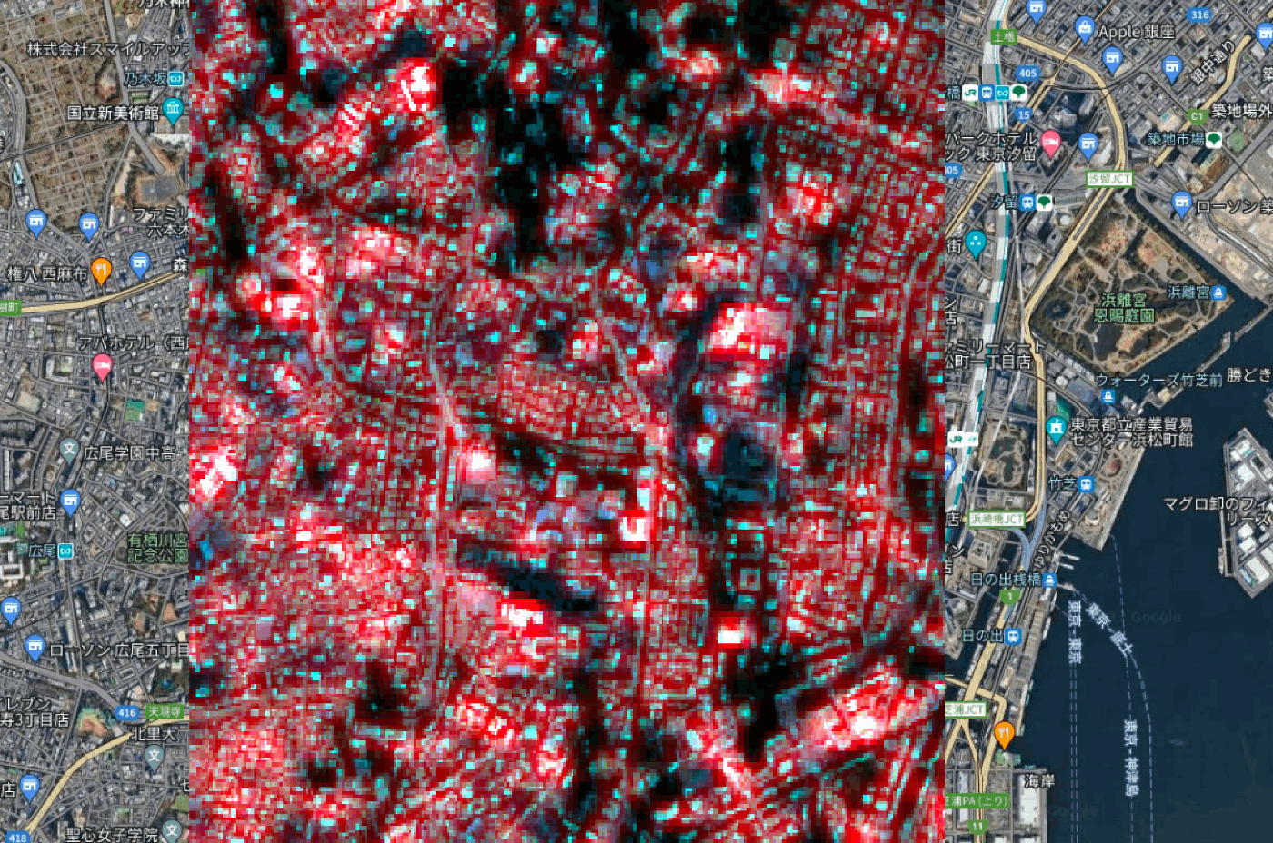
少し拡大すると、
from model import *
from location_encoder import *

model = SatCLIP(
    embed_dim=512,
    image_resolution=224, in_channels=13, vision_layers=4, vision_width=768, vision_patch_size=32, # Image encoder
    le_type='sphericalharmonics', pe_type='siren', legendre_polys=10, frequency_num=16, max_radius=360, min_radius=1, harmonics_calculation='analytic'  # Location encoder
)
こちらでモデルを召喚します。
import tifffile

PATH_TIF = './merge.tif'
img = tifffile.imread(PATH_TIF)[:224, :224]
img.shape # (224, 224, 13)
先ほど加工した衛星画像を読み込ませます。入力サイズは制限します。
img_batch = torch.from_numpy(
    np.stack([img.astype(np.float32), np.zeros((224, 224, 13))], axis=0)
    ).permute(0, 3, 1, 2)
loc_batch = torch.tensor([[139.744421,35.656627],torch.rand((2))])
適当な画像と比較してみます。
with torch.no_grad():
    logits_per_image, logits_per_coord = model(img_batch, loc_batch)
    probs = logits_per_image.softmax(dim=-1).detach().cpu().numpy()

probs
埋め込みの推論を行います。
array([[0.46111405, 0.538886  ],
       [0.62175834, 0.37824163]], dtype=float32)
logits_per_coord.softmax(dim=-1).detach().cpu().numpy()
array([[0.53030545, 0.46969458],
       [0.684439  , 0.31556103]], dtype=float32)
このようにして、画像ごとの類似度の検索と結び付けが可能になります。
cd data/s2
wget https://satclip.z13.web.core.windows.net/satclip/index.csv

cd images
wget https://satclip.z13.web.core.windows.net/satclip/satclip.tar
tar -xf satclip.tar

python clip/main.py
これで学習が可能なようです。
さいごに
最後まで読んでくださってありがとうございます!
画像から位置情報の特定や位置情報との繋ぎ合わせで類似判定が楽になり、検索コストが減るような未来が見えていますね。
衛星データと基盤モデルとの組み合わせが続々と登場しており、新たなソリューションやシステムが展開されていくことを期待しております!
おまけ
こちら以外にも記事執筆をしているのでご参考になれば幸いです
衛星データ解析として、宙畑のライターもしています。
SAR 解析をよくやっていますが、画像系AI、地理空間や衛星データ、点群データに関心があります。
勉強している人は好きなので楽しく絡んでくれると嬉しいです。
Discussion