MyGPT + Math +Julia Code (2)

これは日曜数学 Advent Calendar 2023の25日目の記事です。

はじめに

MyGPT + Math +Julia Code の続きのお話となっています。前回，GPTとのやりとりを紹介しましたが，今回は実際にコードを動かした様子を紹介します。

方程式を解く

$\sin\theta=\cos\theta$を満たす$\theta$

using SymPy

# 変数を定義
x = symbols("x")

# 方程式 sin(x) = cos(x) を定義
eq = Eq(sin(x), cos(x))

# 方程式を解く
solutions = solve(eq, x)

# 解を表示
solutions

$\left[\frac{\pi}4\right]$

グラフを描く

$y=e^x\cos x$のグラフ

using Plots

# 関数を定義
f(x) = exp(x) * cos(x)

# xの範囲を設定
x_vals = -2:0.1:2

# 関数の値を計算
y_vals = f.(x_vals)

# グラフを描く
plot(x_vals, y_vals, label="y = e^x cos(x)", xlabel="x", ylabel="y")

$\sin x+\sin y=\sin(xy)$のグラフ

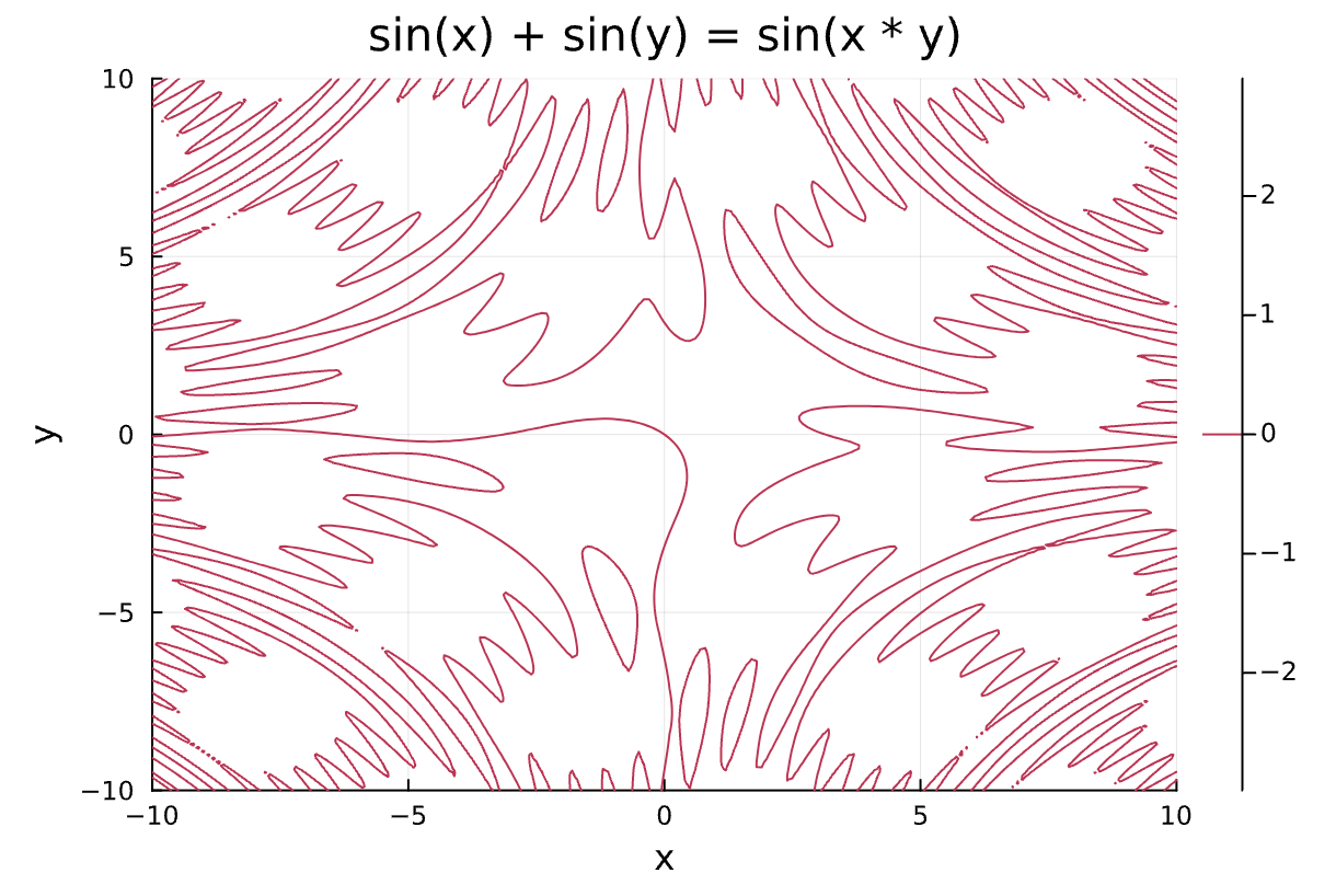
using Plots

# 陰関数を定義
function implicit_func(x, y)
    return sin(x) + sin(y) - sin(x * y)
end

# x と y の範囲を設定
x_vals = -10:0.1:10
y_vals = -10:0.1:10

# 陰関数のコンターを描画
contour(x_vals, y_vals, implicit_func, levels=[0], xlabel="x", ylabel="y", title="sin(x) + sin(y) = sin(x * y)")

$z=\sin x+\sin y$のグラフ

using Plots
plotlyjs() # PlotlyJSバックエンドをアクティブにする
# x と y の範囲を定義
x_vals = -10:0.1:10
y_vals = -10:0.1:10

# z の値を計算する関数
f(x, y) = sin(x) + sin(y)

# 3Dグラフを描画
surface(x_vals, y_vals, f, xlabel="x", ylabel="y", zlabel="z", title="z = sin(x) + sin(y)")

線形代数の計算

行簡約階段形を計算

using RowEchelon

# 行列を定義
A = [1 2 3; 4 5 6; 7 8 9]

# 行簡約階段形を計算
rref_matrix = rref(A)

# 結果を表示
println("Row-Echelon Form of the matrix:")
rref_matrix

Row-Echelon Form of the matrix:

3×3 Matrix{Float64}:
1.0 0.0 -1.0
0.0 1.0 2.0
0.0 0.0 0.0

整数問題

$n$を100以下の自然数とするとき，$n^5 + 5$ と $n^3 + 1$ が互いに素となるようなnの個数を求めてください。

# 互いに素となるnの個数をカウントする変数
count_coprime = 0

# nが1から100までの範囲でループ
for n in 1:100
    # n^5 + 5 と n^3 + 1 の最大公約数を計算
    gcd_value = gcd(n^5 + 5, n^3 + 1)

    # 最大公約数が1なら、互いに素と判断
    if gcd_value == 1
        count_coprime += 1
    end
end

println(count_coprime)

48

πに収束する級数

ライプニッツの公式に基づくπの近似計算関数

$$\pi=4\sum_{n=0}^{\infty}\frac{(-1)^n}{2n+1}$$

using Plots

# ライプニッツの公式に基づくπの近似計算関数
function approximate_pi(n_terms)
    sum = 0.0
    for n in 0:n_terms
        sum += (-1)^n / (2n + 1)
    end
    return 4 * sum
end

# 部分和を計算
n = 1000  # 項の数
partial_sums = [approximate_pi(k) for k in 0:n]

# グラフの作成
plot(0:n, partial_sums, label="πの近似値", color=:blue, linewidth=2)
hline!([π], label="πの実際の値", color=:red, linestyle=:dash)
xlabel!("項の数")
ylabel!("近似値")
title!("ライプニッツの公式によるπの近似")

ラマヌジャンが提案したπの計算に関する公式

$$\pi=\dfrac{2\sqrt2}{9801}\sum_{k=0}^{\infty}\frac{(4k)!(1103+26390k)}{(k!)^4396^{4k}}$$

using SpecialFunctions  # 階乗計算のため

function ramanujan_pi(n_terms)
    total = 0.0
    for k in 0:n_terms-1
        numerator = factorial(big(4*k)) * (1103 + 26390*k)
        denominator = factorial(big(k))^4 * 396^(4*k)
        total += numerator / denominator
    end
    return 1 / (total * (2 * sqrt(2) / 9801))
end

# 最初の数項でのπの近似値
approx_pi = ramanujan_pi(5)  # 5項を使う
approx_pi

3.14159265104104097584529057156622051719404368639054715497847865547777159871135

検定

ある種子の発芽率は従来60%であったが、発芽しやすいよう品種改良した。品種改良した種子から無作為に 600個抽出し種をまいたところ 378個が発芽した。このとき、品種改良によって発芽率が上がったと判断してよいか。有意水準5%で検定せよ。（数研出版　数学B 教科書より）

using Distributions

# 与えられたデータ
n = 600  # 種の数
x = 378  # 発芽した種の数
p_0 = 0.60  # 帰無仮説下の発芽率
alpha = 0.05  # 有意水準

# サンプル発芽率
p_hat = x / n

# 標本比率の標準誤差
SE = sqrt(p_0 * (1 - p_0) / n)

# zスコアの計算
z = (p_hat - p_0) / SE

# 上側の臨界値（一様側検定）
z_critical = quantile(Normal(), 1 - alpha)

# 結果の表示
println("サンプル発芽率 (p_hat): ", p_hat)
println("標本比率の標準誤差 (SE): ", SE)
println("zスコア: ", z)
println("上側臨界値: ", z_critical)

# 検定結果の判断
if z > z_critical
    println("帰無仮説を棄却する（発芽率は60%より高い）")
else
    println("帰無仮説を棄却できない（発芽率が60%より高いとは言えない）")
end

サンプル発芽率 (p_hat): 0.63
標本比率の標準誤差 (SE): 0.02
zスコア: 1.5000000000000013
上側臨界値: 1.6448536269514717
帰無仮説を棄却できない（発芽率が60%より高いとは言えない）

using Distributions
using Plots

# 以前の計算からのデータ
n = 600
x = 378
p_0 = 0.60
alpha = 0.05
p_hat = x / n
SE = sqrt(p_0 * (1 - p_0) / n)
z = (p_hat - p_0) / SE
z_critical = quantile(Normal(), 1 - alpha)

# 標準正規分布の生成
normal = Normal()
x_vals = -3:0.01:3  # zスコアの範囲
y_vals = pdf.(normal, x_vals)  # 正規分布の確率密度関数

# グラフの描画
plot(x_vals, y_vals, label="正規分布", linewidth=2)
vline!([z_critical], label="臨界値", linestyle=:dash, color=:red)
vline!([z], label="zスコア", linestyle=:dash, color=:blue)

# グラフの詳細設定
xlabel!("zスコア")
ylabel!("確率密度")
title!("品種改良による発芽率の統計検定")
plot!(legend=:right)  # legend の位置を指定