GIS × Python Tutorial Session4 ~ geopandas 練習編 ~


はじめに
この記事は「GIS × Python Tutorial」の関連記事です。
今回はgeopandasでのデータ分析を行っていきます。pythonを使用する方であればpandasを使用した事がある方が多いかと思いますので、分からない部分はgeopandasドキュメントを見て行けば躓かずに理解できるかと思います。またgeopandasのgeometryはshapelyのgeometryオブジェクトが入力されるので、個別のメソッドはshapelyの公式ドキュメント、あるいは前回のSession3の記事を参考にしてください。
geopandasとは
geopandasは、pandasの拡張であり、地理空間情報をpandasのDataFrameでデータを扱うことができます。
記事内では以下の事を解説していきます。
- 経緯度からGeoDataFrameを作成する
- CRS関連
- Plotの方法(1) GeoDataFrameの特徴量別に色分けする
- Targetの地点からnメートル以内に含まれるデータを抽出する
- 比較対象区画とgeometryが交差している区画を探す
- 比較対象区画にgeometryが全て含まれている区画を探す
- 比較対象区画とgeometryとで線分を共有している区画を探す
- 比較対象区画にgeometryがn%含まれている区画を探す
- 北側にBufferを作成しその中に含まれているか
- 指定方向に扇状のBufferを作成してその中に存在するか
実行環境
pythonの実行環境はGoogle Colaboratoryを想定しています。 installが必要なライブラリは以下になります
!pip install japanize-matplotlib
Import
# 今回使用するライブラリのインポート
import math
import random
from typing import List

import geopandas as gpd
import japanize_matplotlib
from matplotlib import pyplot as plt
import numpy as np
import pandas as pd
import shapely
from shapely.geometry import LineString, Point, Polygon
from shapely.plotting import plot_polygon, plot_points
plt.style.use('ggplot')
練習編
まずはgeopandasの基本的な使い方から見ていきましょう。
geopandasで最もよく使用するであろうgeopandas.GeoDataFrameはpandas.DataFrameにshapely.geometryが入力された列を追加したものだとイメージしてください。その為shapely.geometryで使用できるモジュールも使用する事が出来ます。
GeoDataFrameとして扱うメリットとしては、shapely.geometryでは単独のオブジェクトデータとしてしか扱う事が出来ませんでしたが、DataFrameなのでオブジェクトと共に様々な特徴量をまとめて管理編集する事が出来ます。shapely.geometryが入力されている列はGeoSeries型のデータとして扱われ、geometryに対する様々なメソッドが用意されており、簡単に全ての行に対して一括処理を行う事が出来ます。
ここで全てを紹介する事はしませんので、気になったモジュールはgeopandas.GeoSeriesのドキュメントを覗いてみてください。
経緯度からGeoDataFrameを作成する
まずは青森県の弘前市にある弘前城をベースとして、適当なデータからGeoDataFrameの作成を行っていきます。
# 弘前城の位置を表すPointのデータを作成する
x = 140.46417575037228
y = 40.60745754283918
base_pt = Point(x, y)

# 適当なPointオブジェクトを複数作成していく
# 適当なデータを作成する
alphabet = 'ABCDEFG'
x_diffs = np.random.normal(0, scale=0.01, size=300)
y_diffs = np.random.normal(0, scale=0.01, size=300)

random_pts = []
names = []
for xd, yd in zip(x_diffs, y_diffs):
    coords = (base_pt.x + xd, base_pt.y + yd)
    pt = Point(coords)
    random_pts.append(pt)
    names.append(alphabet[random.randint(0, 6)])
上記で適当なPointオブジェクトとアルファベットが格納されたリストを作成できました。
実際にGeoDataFrameを作成してみます。
# GeoDataFrameの作成
point_gdf = (
    gpd
    .GeoDataFrame({
        # pandasと同じ様にDict[str, List[Any]]で要素を入力する
        "name": names
    },
    # geometryの引数にList[shapely.geometry]を渡す
    geometry=random_pts,
    # GISなのでCRSも設定しましょう。EPSGコードで設定するのが簡単です。
    crs='EPSG:4326'
    )
)
point_gdf.head(5)
| index | name | geometry |
|---|---|---|
| 0 | E | POINT (140.4600788672616 40.62666668219664) |
| 1 | E | POINT (140.46416605563383 40.59036905443987) |
| 2 | B | POINT (140.472214256954 40.59693754297193) |
| 3 | A | POINT (140.4685266577989 40.63032674640592) |
| 4 | A | POINT (140.46978307504563 40.62772803563662) |
GeoSeriesを作成するならば、geopandas.points_from_xyでPointのオブジェクトが入ったGeoSeriesを作成できます。
# いったんx, yのリストに分ける
x = [p.x for p in random_pts]
y = [p.y for p in random_pts]

_points = gpd.points_from_xy(x=x, y=y, crs='EPSG:4326')
複数のGeoSeriesをDataFrameに
GeoDataFrameではGeoSeriesを複数入力する事も可能です。先ほど作成したGeoDataFrameに弘前城の位置を入れてみましょう。
point_gdf['base'] = (
    gpd
    .GeoSeries(
        [base_pt for _ in range(len(point_gdf))],
        crs='EPSG:4326'
    )
)
point_gdf.head(3)
| index | name | geometry | base |
|---|---|---|---|
| 0 | E | POINT (140.4600788672616 40.62666668219664) | POINT (140.46417575037228 40.60745754283918) |
| 1 | E | POINT (140.46416605563383 40.59036905443987) | POINT (140.46417575037228 40.60745754283918) |
| 2 | B | POINT (140.472214256954 40.59693754297193) | POINT (140.46417575037228 40.60745754283918) |
GeoDataFrameではデフォルトでgeometryの列がジオメトリーの列として設定されていますが、ジオメトリーの列を変更する事も出来ます。
# わかりやすい様に列名を変更する
point_gdf = point_gdf.rename(columns={'geometry': 'random'})

# 列名を変更するとリセットされるので、ジオメトリ―の列を設定する
point_gdf = point_gdf.set_geometry('random')

# ジオメトリ―列の確認
# pandas.DataFrameであれば df.列名 になるがgeopandas.GeoDataFrame
# であればセットされたジオメトリーの列が呼び出されます。
print(point_gdf.geometry.name)
CRS関連
geopandas.GeoDataFrameでは簡単に現在のCRSを調べたり、投影変換する事が出来ます。またUTMのCRSを推定する事も出来ます。
# crsの詳細を表示する
point_gdf.crs
<Geographic 2D CRS: EPSG:4326>
Name: WGS 84
Axis Info [ellipsoidal]:
- Lat[north]: Geodetic latitude (degree)
- Lon[east]: Geodetic longitude (degree)
Area of Use: - name: World.
- bounds: (-180.0, -90.0, 180.0, 90.0)
Datum: World Geodetic System 1984 ensemble - Ellipsoid: WGS 84
- Prime Meridian: Greenwich
# EPSGコードを整数値で取得する
point_gdf.crs.to_epsg()
4326
# UTMの推定
point_gdf.estimate_utm_crs()
<Projected CRS: EPSG:32654>
Name: WGS 84 / UTM zone 54N
Axis Info [cartesian]:
- E[east]: Easting (metre)
- N[north]: Northing (metre)
Area of Use: - name: Between 138°E and 144°E, northern hemisphere between equator and 84°N, onshore and offshore. Japan. Russian Federation.
- bounds: (138.0, 0.0, 144.0, 84.0)
Coordinate Operation: - name: UTM zone 54N
- method: Transverse Mercator
Datum: World Geodetic System 1984 ensemble - Ellipsoid: WGS 84
- Prime Meridian: Greenwich
UTMに投影変換してみましょう。
# 投影変換
point_gdf_utm = point_gdf.to_crs(point_gdf.estimate_utm_crs())
point_gdf_utm.crs
<Projected CRS: EPSG:32654>
Name: WGS 84 / UTM zone 54N
Axis Info [cartesian]:
- E[east]: Easting (metre)
- N[north]: Northing (metre)
Area of Use: - name: Between 138°E and 144°E, northern hemisphere between equator and 84°N, onshore and offshore. Japan. Russian Federation.
- bounds: (138.0, 0.0, 144.0, 84.0)
Coordinate Operation: - name: UTM zone 54N
- method: Transverse Mercator
Datum: World Geodetic System 1984 ensemble - Ellipsoid: WGS 84
- Prime Meridian: Greenwich
この投影変換はgeometryにセットしている列に対してのみ行われます。複数のGeoSeriesを1つのGeoDataFrameとして扱う場合は注意してください。
# 以下の様に投影変換はまとめて行われません。
point_gdf_utm.head(3)
| index | name | random | base |
|---|---|---|---|
| 0 | E | POINT (454336.455457065 4497454.961958681) | POINT (140.46417575037228 40.60745754283918) |
| 1 | E | POINT (454657.6021950703 4493423.714893553) | POINT (140.46417575037228 40.60745754283918) |
| 2 | B | POINT (455343.01633491646 4494148.7196508115) | POINT (140.46417575037228 40.60745754283918) |
baseの方のGeoSeriesも投影変換しておく
# 面倒ですがbaseの方も投影変換します
point_gdf_utm['base'] = (
    point_gdf_utm['base']
    .to_crs(
        point_gdf_utm
        .estimate_utm_crs()
    )
)
point_gdf_utm.head(3)
plotモジュールで特徴量別に色分けしたグラフを作成する
geopandasには簡単にマップを作成できるplotモジュールがあります。shapely.plottingと同じくmatplotlibのFigureオブジェクトを使用する事が出来ます。
plotモジュールの引数には以下のようなものがあります。
- column: str = 色分けに使用する列名を渡す
- cmap: str = カラーマップの名前。
- markersize: int | float = 散布図のマーカーサイズ
- edgecolor: Any = 名前通り
- legend: bool = 凡例を表示するかどうか
- ax: matplotlib.axes._axes.Axes
- missing_kwds: Dict[str, Any] = columnに値が入っていない場合の色などを設定できます。
等をよく使用します。特にmissing_kwdsなどはGISっぽくて個人的に好みです。
おまけ...よく使うColorMap
plt.colormaps.get_cmap('virids')で見られます。
viridis: 個人的に好きでよく使用します

autumn_r: 熱さを表す時に(最後に_rを付けるとcolormapが逆になります)

Blues_r: 寒さを表す時に

coolwarm: 温度を表す時に

Set3: とにかく色々着けたい時に

Plot
上記を参考に実際にPlotしてみます。
base_point_utm = point_gdf_utm.iloc[0]['base']

fig, ax = plt.subplots(figsize=(6, 6))
point_gdf_utm.plot(
    # 色分けする列名を指定する
    column='name',
    cmap='Dark2',
    markersize=5,
    legend=True,
    ax=ax,
)

plot_points(
    base_point_utm,
    color='red',
    ax=ax
)
plt.axis('equal')
plt.show()

空間検索
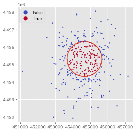
弘前城から1km以内のデータを抽出する
一定範囲内に含まれるデータを抽出する方法は色々ありますが、今回のようなPointを抽出する作業は特に単純で、幾つかの方法があります。
- 1kmのBuffer(Polygon)を作成して範囲内にあるかを調べる
- Pointごとに距離を測り抽出する。
距離を測った方が簡単ですが、ここでは一応2つの方法を書いておきます。
Bufferで抽出する
まずは弘前城から1kmのBufferを作成します。'shapely.geometry.xxx.buffer'と同じ様に使用できます。
# Bufferで抽出する
buff_geom = base_point_utm.buffer(1_000)
方法1.空間検索で抽出する場合
# Buffer内に含まれる行を抽出する
win_buff_gdf = (
    point_gdf_utm[buff_geom.intersects(point_gdf_utm.geometry)]
    .copy()
)
# indexにisinを使用してBool値を入力する
point_gdf_utm['win_buff'] = (
    point_gdf_utm
    .index
    .isin(win_buff_gdf.index)
)
point_gdf_utm[['name', 'win_buff']].head(3)
| index | name | win_buff |
|---|---|---|
| 0 | A | false |
| 1 | G | false |
| 2 | E | true |
方法2.距離で抽出する場合
point_gdf_utm['win_buff'] = (
    np.where(
        point_gdf_utm['base'].distance(point_gdf_utm['random']) <= 1_000,
        True,
        False
    )
)
geopandasにはsjoin(spatial join: 空間結合)もありますが、pandasのjoinメソッドの挙動が個人的にあまり好きではないのでここでは使用しませんでした。
Plotしてみましょう。
fig, ax = plt.subplots(figsize=(5, 5))
plot_polygon(
    buff_geom,
    add_points=False,
    fill=None,
    lw=2,
    ax=ax
)
point_gdf_utm.plot(
    column='win_buff',
    cmap='coolwarm',
    markersize=6,
    legend=True,
    ax=ax
)
plt.axis('equal');
空間検索についてもう少し
空間検索や空間結合はGISではよく使用するGISらしさのある機能です。
今まではPointのデータを対象としていたのであまり考える必要がありませんでしたが、PolygonやLineStringを使用する場合はもう少し考える必要があります。例でいうと
- 比較対象のPolygonに触れている(True | False)
- 比較対象のPolygon内に全て含まれているか(True | False)
- 比較対象のPolygonと線分を共有しているか(True | False)
- 比較対象のPolygon内にn%以上含まれているか(True | False)
などが考えられます。上記のリストを1つずつ考えてみましょう。
geojson
geoj = """{
  "type": "FeatureCollection",
  "features": [
    {
      "type": "Feature",
      "properties": {
        "name": "メインの区画"
      },
      "geometry": {
        "type": "Polygon",
        "coordinates": [
          [
            [
              140.461482,
              40.605913
            ],
            [
              140.462029,
              40.612421
            ],
            [
              140.471385,
              40.61247
            ],
            [
              140.471234,
              40.605954
            ],
            [
              140.461482,
              40.605913
            ]
          ]
        ]
      }
    },
    {
      "type": "Feature",
      "properties": {
        "name": "触れていない区画"
      },
      "geometry": {
        "type": "Polygon",
        "coordinates": [
          [
            [
              140.462394,
              40.605213
            ],
            [
              140.46249,
              40.603502
            ],
            [
              140.464228,
              40.604643
            ],
            [
              140.462394,
              40.605213
            ]
          ]
        ]
      }
    },
    {
      "type": "Feature",
      "properties": {
        "name": "少しだけ触れている区画"
      },
      "geometry": {
        "type": "Polygon",
        "coordinates": [
          [
            [
              140.467222,
              40.605457
            ],
            [
              140.467393,
              40.606329
            ],
            [
              140.474957,
              40.605229
            ],
            [
              140.469657,
              40.603364
            ],
            [
              140.467222,
              40.605457
            ]
          ]
        ]
      }
    },
    {
      "type": "Feature",
      "properties": {
        "name": "半分以上触れている区画"
      },
      "geometry": {
        "type": "Polygon",
        "coordinates": [
          [
            [
              140.469368,
              40.611224
            ],
            [
              140.469067,
              40.607697
            ],
            [
              140.472254,
              40.607779
            ],
            [
              140.469368,
              40.611224
            ]
          ]
        ]
      }
    },
    {
      "type": "Feature",
      "properties": {
        "name": "全て含まれる区画"
      },
      "geometry": {
        "type": "Polygon",
        "coordinates": [
          [
            [
              140.463735,
              40.611696
            ],
            [
              140.463606,
              40.610483
            ],
            [
              140.466256,
              40.610458
            ],
            [
              140.46646,
              40.611656
            ],
            [
              140.463735,
              40.611696
            ]
          ]
        ]
      }
    },
    {
      "type": "Feature",
      "properties": {
        "name": "線分を共有している区画_1"
      },
      "geometry": {
        "type": "Polygon",
        "coordinates": [
          [
            [
              140.461482,
              40.605913
            ],
            [
              140.462029,
              40.612421
            ],
            [
              140.461185,
              40.61247
            ],
            [
              140.461482,
              40.605913
            ]
          ]
        ]
      }
    },
    {
      "type": "Feature",
      "properties": {
        "name": "線分を共有している区画_2"
      },
      "geometry": {
        "type": "Polygon",
        "coordinates": [
          [
            [
              140.462029,
              40.612421
            ],
            [
              140.471385,
              40.61247
            ],
            [
              140.462029,
              40.613954
            ],
            [
              140.462029,
              40.612421
            ],
          ]
        ]
      }
    },
  ]
}"""
まずはGeoDataFrameを作成します。
poly_gdf = gpd.read_file(geoj)
poly_gdf = poly_gdf.set_crs(crs='EPSG:4326')
poly_gdf = poly_gdf.to_crs(poly_gdf.estimate_utm_crs())
| index | name |
|---|---|
| 0 | メインの区画 |
| 1 | 触れていない区画 |
| 2 | 少しだけ触れている区画 |
| 3 | 半分以上触れている区画 |
| 4 | 全て含まれる区画 |
| 5 | 線分を共有している区画_1 |
| 6 | 線分を共有している区画_2 |

前準備としてメインとそれ以外で分けておきます
main_poly = poly_gdf.iloc[0].geometry
sub_polys = poly_gdf.iloc[1: ].copy()
メイン区画と交差している区画を探す
まずはgeometry同士が交差しているか(含まれている場合も)を判定します。
GeoSeries.intersectsモジュールを使用しましょう。
# Bool値を入力する場合
sub_polys['intersects'] = sub_polys.intersects(main_poly)
# 抽出する場合
_sub_polys = sub_polys[sub_polys.intersects(main_poly)].copy()
| index | name | intersects |
|---|---|---|
| 1 | 触れていない区画 | false |
| 2 | 少しだけ触れている区画 | true |
| 3 | 半分以上触れている区画 | true |
| 4 | 全て含まれる区画 | true |
| 5 | 線分を共有している区画_1 | true |
| 6 | 線分を共有している区画_2 | true |
メイン区画に完全に含まれてる区画を探す
次にgeometryが全て含まれている場合を判定します。
# Bool値を入力する場合
sub_polys['within'] = sub_polys.within(main_poly)

# 抽出する場合
_sub_polys = sub_polys[sub_polys.within(main_poly)].copy()
| index | name | intersects | within |
|---|---|---|---|
| 1 | 触れていない区画 | false | false |
| 2 | 少しだけ触れている区画 | true | false |
| 3 | 半分以上触れている区画 | true | false |
| 4 | 全て含まれる区画 | true | true |
| 5 | 線分を共有している区画_1 | true | false |
| 6 | 線分を共有している区画_2 | true | false |
線分を共有している区画を探す
比較対象のgeometryと共通の部分を持ち、交差していないgeometryを探します。
例えば青森県を比較対象とした場合は秋田県と岩手県が線分を共有していると言えますし、北海道は線分を共有している都道府県はないと言えます。
# Bool値を入力する場合
sub_polys['touches'] = sub_polys.touches(main_poly)

# 抽出する場合
_sub_polys = sub_polys[sub_polys.touches(main_poly)].copy()
| index | name | intersects | within | touches |
|---|---|---|---|---|
| 1 | 触れていない区画 | false | false | false |
| 2 | 少しだけ触れている区画 | true | false | false |
| 3 | 半分以上触れている区画 | true | false | false |
| 4 | 全て含まれる区画 | true | true | false |
| 5 | 線分を共有している区画_1 | true | false | true |
| 6 | 線分を共有している区画_2 | true | false | true |
メイン区画にn%含まれる区画を探す
上記のようなモジュールはないので(多分、ドキュメントで見落としがなければ)自分で作成する必要があります。しかし似た計算が可能なモジュールがあるので実際に挙動を確認してみましょう。
必要な事は
- 比較対象のPolygonの面積を計算する
- 比較対象と重なっている部分の面積を計算する
- 面積の比を求める
上記で求められます。今回は関数にしてしまいましょう。
def within_ratio(
    main_poly: Polygon,
    gdf: gpd.GeoDataFrame,
    ratio: float=0.5,
    res_bool: bool=False
) -> List[float] | List[bool]:
    df = gdf.copy()
    # 比較対象の面積
    area = df.geometry.area
    # intersectionで含まれている部分のgeometryを取得する
    within_area = gdf.geometry.intersection(main_poly).area
    # 比を計算する
    with_in_ratio = within_area / area
    if res_bool:
        func = lambda x: True if ratio <= x else False
        return [func(_area) for _area in with_in_ratio]
    else:
        return with_in_ratio.to_list()
sub_polys['within_ratio'] = (
    within_ratio(
        main_poly=main_poly,
        gdf=sub_polys,
        ratio=0.5,
        res_bool=True
    )
)
| index | name | intersects | within | touches | within_ratio |
|---|---|---|---|---|---|
| 1 | 触れていない区画 | false | false | false | false |
| 2 | 少しだけ触れている区画 | true | false | false | false |
| 3 | 半分以上触れている区画 | true | false | false | true |
| 4 | 全て含まれる区画 | true | true | false | true |
| 5 | 線分を共有している区画_1 | true | false | true | false |
| 6 | 線分を共有している区画_2 | true | false | true | false |
ほかにも色々とありますので、気になった方はGeoSeriesのBinary predicatesを覗いてみてください。
ちょっと変わった空間検索
ある地点から一定方向に範囲を設定して、そこに含まれるかを調べてみましょう。
北側にBufferを作成してその中に存在するか
弘前城から真北の0度方向に2000m×500mの帯を作成しその中に存在するかを調べます。
まずはベースとなるPointオブジェクトから距離と真北の方位角から新たなPointを取得する関数を作成します。
def to_point(base_point, distance, angle):
    # 距離と方向から新しいPointObjectを作成する
    angle_rad = math.radians(angle)
    x = base_point.x + distance * math.sin(angle_rad)
    y = base_point.y + distance * math.cos(angle_rad)
    destination = (x, y)
    return Point(destination)
実際に動作させてみましょう。
弘前城から真北に2000m進んだ場所にPointを作成し、そこまでをLineStringで繋ぎます。その線からBufferを作成し、Bufferと交差しているPointにBool値を入力します。
# 弘前城から真北方向に2000m進んだ場所のPointを作成する
to_pt = to_point(
    base_point=base_point,
    distance=2_000,
    angle=0
)

# 2000m×500mのBufferを作成する
north_buff = (
    LineString([base_point, to_pt])
    .buffer(500, cap_style='flat')
)

# 経緯度のgdfはもう使用しないので、余計な列を削除するついでに上書きする。
point_gdf = point_gdf_utm.drop(['base', 'win_buff'], axis=1)
point_gdf['within_north_buff'] = point_gdf.intersects(north_buff)
| index | name | random | within_north_buff |
|---|---|---|---|
| 0 | A | POINT (455806.1954772188 4495307.418559175) | false |
| 1 | G | POINT (455683.6708025543 4495307.132798844) | false |
| 2 | E | POINT (454814.1940392553 4495087.460774167) | false |
| 3 | G | POINT (454498.59814017836 4495980.257076586) | true |
| 4 | C | POINT (454662.6950009358 4496949.4123351155) | true |

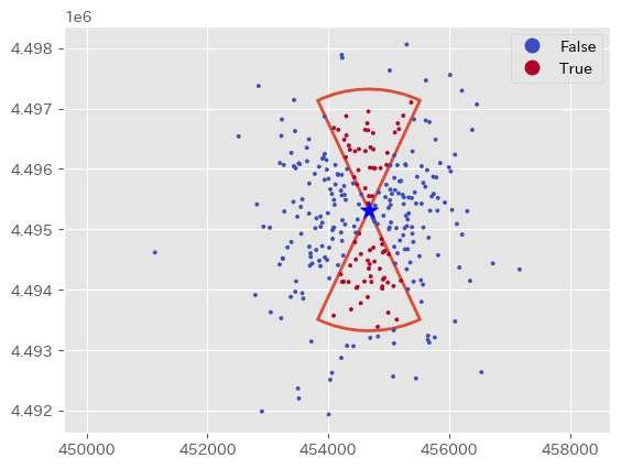
扇状のBufferを作成してその中に存在するか
弘前城から2000mのBufferを作成し、北側335度から25度までの間、南側165度から205度の間に存在するかを調べます。
例えば空港の侵入方向などに関連するオブジェクトを探す時などに使用出ます。
まずはベースとなるPointオブジェクトから距離と2つの方位角を使用して扇型のPolygonを作成する関数を作成しましょう。
def directional_fan(base_point, distance, angle1, angle2):
    buff = base_point.buffer(distance)
    pt1 = to_point(base_point, distance * 2, angle1)
    pt2 = to_point(base_point, distance * 2, angle2)
    triangle = Polygon([base_point, pt1, pt2])
    target = buff.intersection(triangle)
    return target
実際に動作させてみます。
# 北側の範囲を作成します。
north_fan_buff = directional_fan(
    base_point=base_point,
    distance=2000,
    angle1=335,
    angle2=25
)
# 南側の範囲を作成します。
south_fan_buff = directional_fan(
    base_point=base_point,
    distance=2000,
    angle1=155,
    angle2=205
)

# unionモジュールを使用して、二つの扇形のPolygonを結合します。
fan_buff = north_fan_buff.union(south_fan_buff)
# Bool値の入力
point_gdf['within_fan_buff'] = point_gdf.intersects(fan_buff)
| index | name | random | within_north_buff | within_fan_buff |
|---|---|---|---|---|
| 0 | A | POINT (455806.1954772188 4495307.418559175) | false | false |
| 1 | G | POINT (455683.6708025543 4495307.132798844) | false | false |
| 2 | E | POINT (454814.1940392553 4495087.460774167) | false | false |
| 3 | G | POINT (454498.59814017836 4495980.257076586) | true | true |
| 4 | C | POINT (454662.6950009358 4496949.4123351155) | true | true |
おわりに
いかがだったでしょうか。本当は実際のデータも使用したかったのですが、長くなったので実践編は後日という事で...
実践編では実際のデータを使用して、GISらしい地理的な特徴を利用した考える事が出来るMapを作成する方法をメインに書いていこうと思っています。
Discussion