🙆♀️
cmdstanpy : スパースモデル


import os
import time

import pandas as pd
import matplotlib.pyplot as plt
import seaborn as sns
from sklearn.datasets import make_regression
from cmdstanpy import CmdStanModel
データの読み込み
以下のデータを使用しています。
x, y, true_coef = make_regression(random_state=12,
                       n_samples=100,
                       n_features=10,
                       n_informative=4,
                       noise=10.0,
                       bias=0.0,
                       coef=True)
print(true_coef)
[57.11877412  0.          6.5277752   0.          0.         85.58078808
  0.          0.          0.         56.5335269 ]
df = pd.DataFrame(x)
df['y'] = y
Bayesian Lasso
こちらを参考にしました。
回帰係数の事前分布として二重指数分布を採用することで実装できます。
lasso.stan
// ref: https://blog.atusy.net/2022/01/09/bayesian-lasso/
data {
    // 入力のチェックにもなるのでわかるところは下限と上限をつける
    int<lower=0> N;
    int<lower=0> K;
    matrix[N, K] X;
    vector[N] y;
}

parameters {
    real alpha;
    vector[K] beta;
    real<lower=0> sigma;
    real<lower=0> b;
}

transformed parameters {
    vector[N] mu;
    mu = alpha + X*beta;
}

model {
    // 重み(beta)の事前分布として二重指数分布を指定
    beta ~ double_exponential(0, b);

    // 各パラメータの無情報事前分布の指定は省略
    y ~ normal(mu, sigma);
}

generated quantities {
    /* 各サンプルの予測分布を得るために、ここで正規分布から乱数を発生させて計算 */
    array[N] real y_pred;
    y_pred = normal_rng(mu, sigma);
}
馬蹄事前分布を使用した回帰モデル
こちらを参考にしました。
Bayesian Lassoの事後中央値は0の値とならないことが欠点としてある(参考)ため、
回帰係数の事前分布として馬蹄事前分布をを採用することで実装できます。
horse.stan
// ref: https://web.archive.org/web/20160405001356/https://ariddell.org/horseshoe-prior-with-stan.html
data {
    // 入力のチェックにもなるのでわかるところは下限と上限をつける
    int<lower=0> N;
    int<lower=0> K;
    matrix[N, K] X;
    vector[N] y;
}

parameters {
    real alpha;
    vector[K] beta;
    real<lower=0> sigma;
    vector<lower=0>[K] lambda;
    real<lower=0> tau;
}

transformed parameters {
    vector[N] mu;
    mu = alpha + X*beta;
}

model {
    // 重み(beta)の事前分布として馬蹄分布を指定
    lambda ~ cauchy(0, 1);
    tau ~ cauchy(0, 1);
    for (k in 1:K) {
        beta[k] ~ normal(0, lambda[k]*tau);
    }

    // 各パラメータの無情報事前分布の指定は省略
    y ~ normal(mu, sigma);
}

generated quantities {
    /* 各サンプルの予測分布を得るために、ここで正規分布から乱数を発生させて計算 */
    array[N] real y_pred;
    y_pred = normal_rng(mu, sigma);
}
output_dir = "./output/"
os.makedirs(output_dir, exist_ok=True)

lasso_stan_file = "./lasso.stan"
lasso_exe_file = "./lasso"

horse_stan_file = "./horse.stan"
horse_exe_file = "./horse"
コンパイル
if not os.path.exists(lasso_exe_file):
    lasso_model = CmdStanModel(stan_file=lasso_stan_file)
else:
    lasso_model = CmdStanModel(exe_file=lasso_exe_file)
16:55:45 - cmdstanpy - INFO - compiling stan file /Users/yyamaguchi/Desktop/programming/BayesianStatistics/src/04_sparse/lasso.stan to exe file /Users/yyamaguchi/Desktop/programming/BayesianStatistics/src/04_sparse/lasso
16:55:50 - cmdstanpy - INFO - compiled model executable: /Users/yyamaguchi/Desktop/programming/BayesianStatistics/src/04_sparse/lasso
if not os.path.exists(horse_exe_file):
    horse_model = CmdStanModel(stan_file=horse_stan_file)
else:
    horse_model = CmdStanModel(exe_file=horse_exe_file)
17:04:02 - cmdstanpy - INFO - compiling stan file /Users/yyamaguchi/Desktop/programming/BayesianStatistics/src/04_sparse/horse.stan to exe file /Users/yyamaguchi/Desktop/programming/BayesianStatistics/src/04_sparse/horse
17:04:08 - cmdstanpy - INFO - compiled model executable: /Users/yyamaguchi/Desktop/programming/BayesianStatistics/src/04_sparse/horse
データ
data = {
    "N": len(df),
    "K": 10,
    "X": df.drop("y", axis=1).values,
    "y": df["y"].values,
}
フィッティング
CmdStanPyでは以下のsample()メソッドにより、ハミルトンモンテカルロ(HMC)サンプリングを使って、データを条件としたモデルに対するベイズ推定を行います。このメソッドは、モデルとデータに対してStanのHMC-NUTSサンプラーを実行し、CmdStanMCMCオブジェクトを返します。
データは以下のようにPythonの辞書型でも渡せますし、ファイルパスを渡すこともできます。
import multiprocessing
num_cpu = multiprocessing.cpu_count()
lasso_fit = lasso_model.sample(
    data=data,
    chains=4, # chain数
    seed=1, # seed固定
    iter_warmup=1000, # warmupの数
    iter_sampling=2000, # samplingの数
    parallel_chains=num_cpu, # 並列数
    save_warmup=True, # warmupもCSVに保存
    thin=1, # サンプリング間隔
    output_dir=output_dir, # 出力先
    # show_console=True, # 標準出力
    show_progress=True # progress出力
    )
17:04:50 - cmdstanpy - INFO - Requested 8 parallel_chains but only 4 required, will run all chains in parallel.
17:04:50 - cmdstanpy - INFO - CmdStan start processing


chain 1 |          | 00:00 Status


chain 2 |          | 00:00 Status


chain 3 |          | 00:00 Status


chain 4 |          | 00:00 Status


17:04:51 - cmdstanpy - INFO - CmdStan done processing.
17:04:51 - cmdstanpy - WARNING - Non-fatal error during sampling:
Exception: double_exponential_lpdf: Scale parameter is inf, but must be positive finite! (in '/Users/yyamaguchi/Desktop/programming/BayesianStatistics/src/04_sparse/lasso.stan', line 24, column 4 to column 36)
Exception: double_exponential_lpdf: Scale parameter is inf, but must be positive finite! (in '/Users/yyamaguchi/Desktop/programming/BayesianStatistics/src/04_sparse/lasso.stan', line 24, column 4 to column 36)
Consider re-running with show_console=True if the above output is unclear!
horse_fit = horse_model.sample(
    data=data,
    chains=4, # chain数
    seed=1, # seed固定
    iter_warmup=1000, # warmupの数
    iter_sampling=2000, # samplingの数
    parallel_chains=num_cpu, # 並列数
    save_warmup=True, # warmupもCSVに保存
    thin=1, # サンプリング間隔
    output_dir=output_dir, # 出力先
    # show_console=True, # 標準出力
    show_progress=True # progress出力
    )
17:09:38 - cmdstanpy - INFO - Requested 8 parallel_chains but only 4 required, will run all chains in parallel.
17:09:38 - cmdstanpy - INFO - CmdStan start processing


chain 1 |          | 00:00 Status


chain 2 |          | 00:00 Status


chain 3 |          | 00:00 Status


chain 4 |          | 00:00 Status


17:09:39 - cmdstanpy - INFO - CmdStan done processing.
17:09:39 - cmdstanpy - WARNING - Non-fatal error during sampling:
Exception: normal_lpdf: Scale parameter is 0, but must be positive! (in '/Users/yyamaguchi/Desktop/programming/BayesianStatistics/src/04_sparse/horse.stan', line 28, column 8 to column 43)
Consider re-running with show_console=True if the above output is unclear!
17:09:39 - cmdstanpy - WARNING - Some chains may have failed to converge.
	Chain 1 had 129 divergent transitions (6.5%)
	Chain 2 had 178 divergent transitions (8.9%)
	Chain 3 had 171 divergent transitions (8.6%)
	Chain 4 had 141 divergent transitions (7.0%)
	Use function "diagnose()" to see further information.
結果の確認
fit.summary()で各パラメータの要約が見られます。lp__は対数事後確率で他のパラメータ同様に収束する必要があります。
また、N_EffはStanが自己相関等から判断した実効的なMCMCサンプル数です。この数が少ないと収束しづらいパラメータであることが分かります。大体1000サンプルほどあると良いものです。
lasso_fit.summary().head(14)
horse_fit.summary().head(14)
arvizによる収束性判断
import numpy as np
import arviz as az
import xarray as xr
az.style.use("arviz-darkgrid")
cmdstanpyからarviz用のデータへ変換
lasso_cmdstanpy_data = az.from_cmdstanpy(
    posterior=lasso_fit,
    log_likelihood="lp__",
)
lasso_cmdstanpy_data
horse_cmdstanpy_data = az.from_cmdstanpy(
    posterior=horse_fit,
    log_likelihood="lp__",
)
horse_cmdstanpy_data
事後分布のプロット
馬蹄事前分布を使用した回帰モデルの方がBayesian Lassoと比較して事後平均の値が0に近くなっていることや標準偏差が小さいことがわかります。
az.plot_posterior(lasso_cmdstanpy_data, var_names=["alpha", "beta", "sigma"]);

az.plot_posterior(horse_cmdstanpy_data, var_names=["alpha", "beta", "sigma"]);

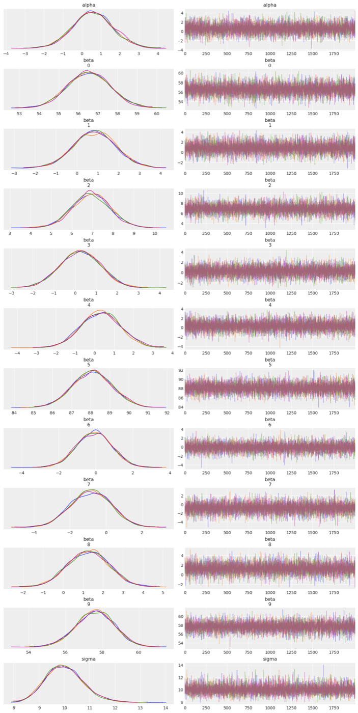
トレースプロット
馬蹄事前分布を使用した回帰モデルの方が収束性が悪そうですね。
az.plot_trace(lasso_cmdstanpy_data, compact=False, var_names=["alpha", "beta", "sigma"]);
az.plot_trace(horse_cmdstanpy_data, compact=False, var_names=["alpha", "beta", "sigma"]);

Discussion